Determinants of House Prices in Sidney, Australia
VerifiedAdded on 2023/05/28
|18
|3308
|305
AI Summary
This research identifies the major determinants of house prices in Sidney, Australia using simple random sampling method. The findings show that the size of land, house price index, annual price change, and age of the house are the major determinants of house prices in Sidney.
Contribute Materials
Your contribution can guide someone’s learning journey. Share your
documents today.
Statistics for financial decisions
Statistics for Financial Decisions
Student name:
Tutor name:
1 | P a g e
Statistics for Financial Decisions
Student name:
Tutor name:
1 | P a g e
Secure Best Marks with AI Grader
Need help grading? Try our AI Grader for instant feedback on your assignments.
Statistics for financial decisions
Executive summary
The main objective of this research was to identify the major determinants of prices of
houses in the city of Sidney in Australia. The size of land in square meters, house price
index, annual price change and age of the house were identified as the major
determinants of the house prices in the city. This research employed simple random
sampling method where a sample of 15 years was selected. Analysis was carried out
through the use of excel after which the findings were presented in form of tables and
graphs. It was found that the price of houses in Sidney was affected differently by the
house price determinants. Housing price index was found to have the strongest
influence on the house market price while the size of land in square meters was found
to have the least influence on the price of houses. To add on, the research discovered
that all the variables had a positive relationship with the house price except the age of
the house in years which depicted a negative relationship.
2 | P a g e
Statistics for financial decisions
Introduction
Housing prices in the real estate industry have been seen to fluctuate in the recent
decade globally (Dongsheng & Zhong, 2010). This has been confirmed by the house
price trend in many cities of the world. Australia’s housing prices have not been any
different. To be specific, the city of Sidney has witnessed increased house prices. This
has been caused by proximity to the city, forces of demand and supply among others
(Hua, 2008) and (Shisong & Hongmei, 2009). Less research has been conducted on the
factors affecting housing prices in Sidney therefore it is difficult to attribute this price
increase to any factor. However, some of the evident factors affecting house prices in
Sidney include the size of land the house is lying on, housing price index and annual
percentage change
This research study is focused in creating a model that will be used to predict the house
prices in Sidney using the above named variables. For example, the age of the house
would be a major component of the model since new houses are likely to fetch high
prices due to high demand while old houses are likely to fetch lower prices due to low
demand (Nellis, 2011). Another major component of the model will be the size of land
on which the house is built (Abelson & Chung, 2005). It is normal that a house sitting on
a large area will go at a higher price while a house sitting on a smaller size of land will
fetch a lower price in a given area (Quigley , 2009).
3 | P a g e
Statistics for financial decisions
LITERATURE REVIEW
The last decade has witnessed a soar in the house prices in Sidney. According to a
research done by (Haurin & Gill, 2012), in 2003, the median house price in Sidney was
about 473 dollars. About 11 years later in mid-2014, the median price had shot to
811,000 dollars. This is an increase of 70%. According Real Estate Institute of Australia
(REIA), the data indicated stability between the year 1990 and 1999. However, an
increase was witnessed in the year 2000. The scenario was even worse during the
global financial crisis of 2007/2008 as there was a steady increase. In 2014, a research
conducted by demographics 10th annual survey compared the ratio of family income to
median house prices in Australia. The research found that Australia had a very high
mean house income price in comparison to developed economies of the world such as
japan, UK and US (Karantonis & Ge, 2007).
METHODOLOGY
Data collection
The data used in this study was shared by the Australian Bureau of Statistics. This was
under residential property prices. The information gathered included the house values in
thousand dollars, the number of years that the houses had stayed the size of land, price
index of the city and yearly percentage change in real estate values. The sampling
method used by the study to select the years from the year 2002 to 2017 was
judgmental sampling where a convenient sample was used. The recent last 15 years
were picked for the study. The variables involved in this research study were all
numerical variables thereby prompting the use of quantitative analysis. There were both
4 | P a g e
Secure Best Marks with AI Grader
Need help grading? Try our AI Grader for instant feedback on your assignments.
Statistics for financial decisions
dependent and independent variables. The dependent variable was the house market
price while the independent variables were age of the houses, size of land in square
meters, price index and annual percentage change.
Data analysis
The research employed quantitative statistics in the analysis of the data. Both inferential
and descriptive statistics were conducted. Descriptive statistics involved establishing
measures of center as well as measures of dispersion. Measures of central tendency
such as mean, mode and median were established. Measures of dispersion such as
standard deviation and variance were also calculated. Inferential statistics such as
correlation and regression analysis were conducted to establish how dependent
variable related with the independent variables. The results were mainly presented in
form of tables and graphs for clear interpretation. For the sake of the main objective of
this study, simple linear regression and multiple linear regression was established to
identify the best model that could be used to predict the house prices in the city of
Sidney with a lot of precision.
Limitations
The major limitation in this research study was the fact that there was no enough time
for data collection all the way to compiling of the report. This made the study to be
rushed which could impact negatively on the results. There was also a problem of
multicollinearity when it came to data analysis.
5 | P a g e
Statistics for financial decisions
ANALYSIS AND FINDINGS
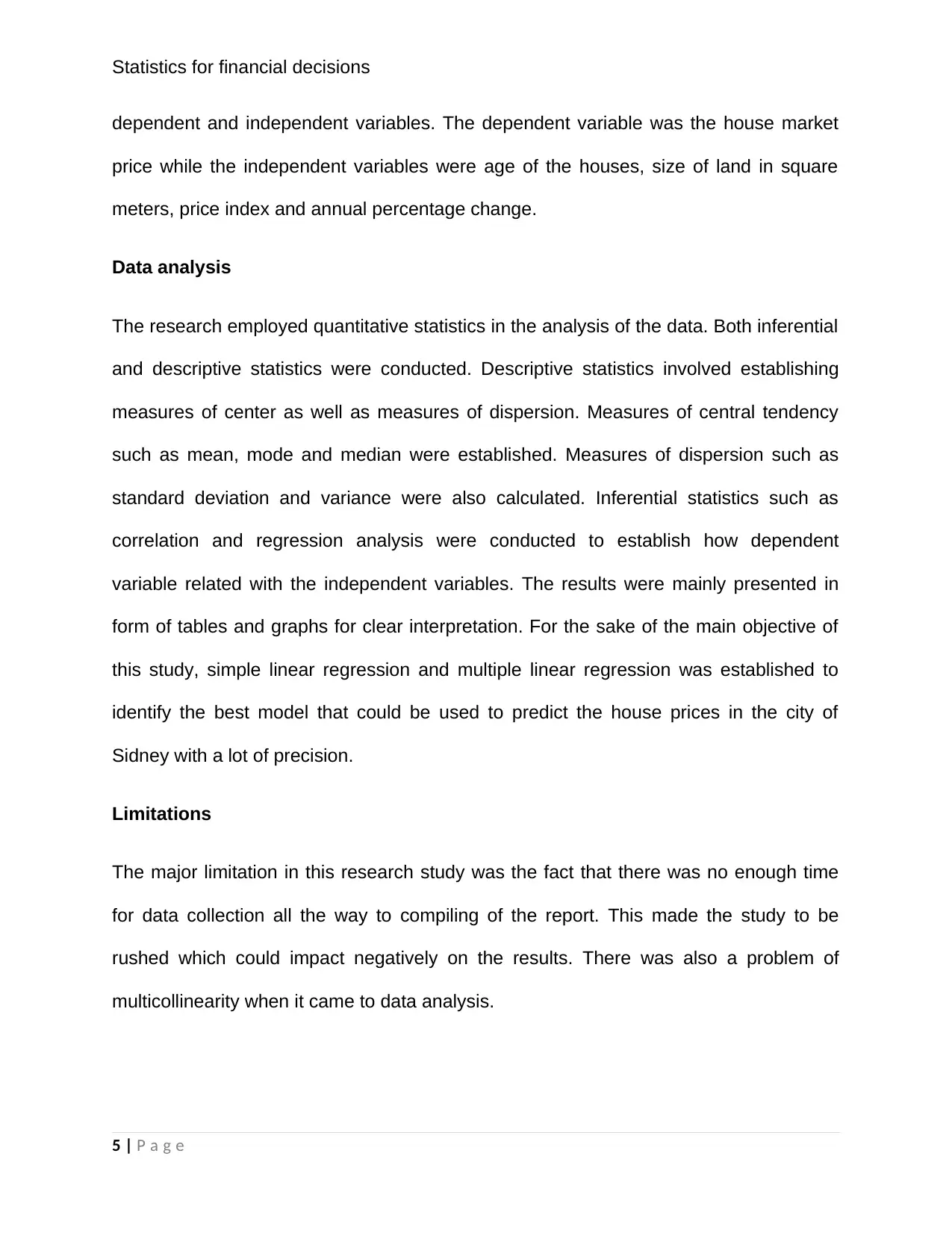
1. Summary - Market price of houses in Sidney
Market Price ($000)
Mean 777
Standard Error 20.9295
9
Median 780
Mode #N/A
Standard
Deviation
81.0599
4
Sample Variance 6570.71
4
Kurtosis 1.13610
6
Skewness 0.17849
2
Range 330
Minimum 630
Maximum 960
Count 15
Table 1. Source: Research project
The summary statistics is of market price of houses in Sidney. The analysis results
show that the average house price in thousand dollars was 777 dollars. The minimum
house price in thousand dollars was 630 dollars while the maximum house price in
thousand dollars was 960 dollars. The median price in thousand dollars was 780
dollars.
6 | P a g e
ANALYSIS AND FINDINGS
1. Summary - Market price of houses in Sidney
Market Price ($000)
Mean 777
Standard Error 20.9295
9
Median 780
Mode #N/A
Standard
Deviation
81.0599
4
Sample Variance 6570.71
4
Kurtosis 1.13610
6
Skewness 0.17849
2
Range 330
Minimum 630
Maximum 960
Count 15
Table 1. Source: Research project
The summary statistics is of market price of houses in Sidney. The analysis results
show that the average house price in thousand dollars was 777 dollars. The minimum
house price in thousand dollars was 630 dollars while the maximum house price in
thousand dollars was 960 dollars. The median price in thousand dollars was 780
dollars.
6 | P a g e
Statistics for financial decisions
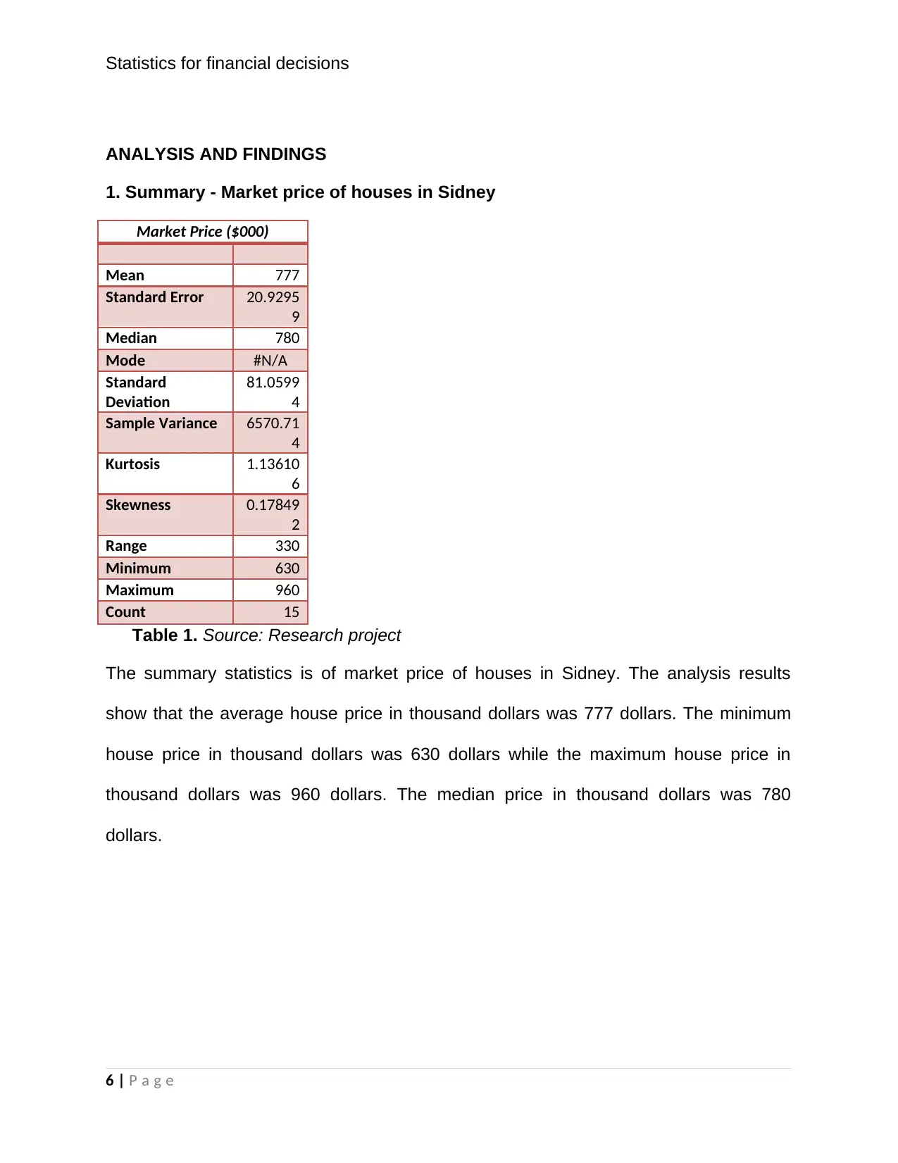
3. House market price trend in Sidney from 2002 to 2017
Figure 1. Source: Research project
The time series graph above indicates how the house price has been moving since the
year 2002 to the year 2017. There is a gentle slope meaning that the price has been
increasing gradually from one year to another.
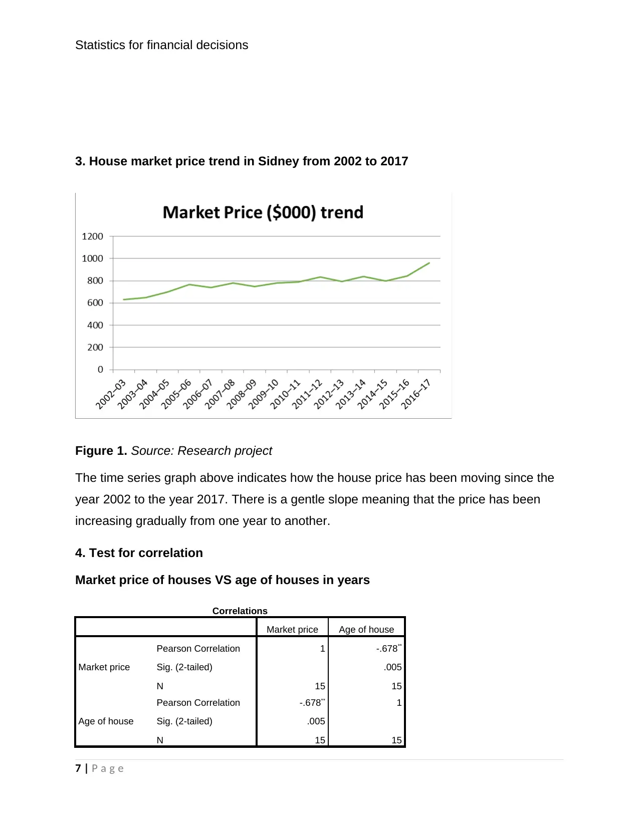
4. Test for correlation
Market price of houses VS age of houses in years
Correlations
Market price Age of house
Market price
Pearson Correlation 1 -.678**
Sig. (2-tailed) .005
N 15 15
Age of house
Pearson Correlation -.678** 1
Sig. (2-tailed) .005
N 15 15
7 | P a g e
3. House market price trend in Sidney from 2002 to 2017
Figure 1. Source: Research project
The time series graph above indicates how the house price has been moving since the
year 2002 to the year 2017. There is a gentle slope meaning that the price has been
increasing gradually from one year to another.
4. Test for correlation
Market price of houses VS age of houses in years
Correlations
Market price Age of house
Market price
Pearson Correlation 1 -.678**
Sig. (2-tailed) .005
N 15 15
Age of house
Pearson Correlation -.678** 1
Sig. (2-tailed) .005
N 15 15
7 | P a g e
Paraphrase This Document
Need a fresh take? Get an instant paraphrase of this document with our AI Paraphraser
Statistics for financial decisions
**. Correlation is significant at the 0.01 level (2-tailed).
Table 2. Source: Research project
From the correlation analysis above, it can be observed that there is a strong relationship between
market house prices and the age of the houses. However, the relationship is in the negative
direction. Statistically, the correlation was found to be significant since the p-value is less than
0.05.
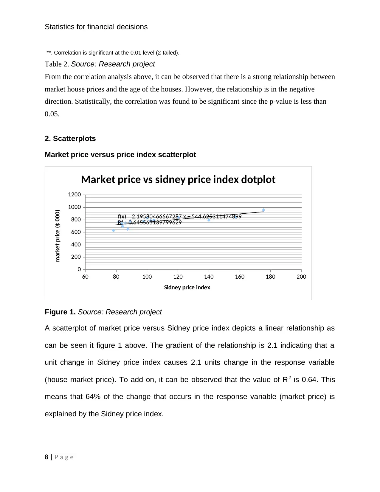
2. Scatterplots
Market price versus price index scatterplot
60 80 100 120 140 160 180 200
0
200
400
600
800
1000
1200
f(x) = 2.19580466667287 x + 544.625311474899
R² = 0.645565139799629
Market price vs sidney price index dotplot
Sidney price index
market price ($ 000)
Figure 1. Source: Research project
A scatterplot of market price versus Sidney price index depicts a linear relationship as
can be seen it figure 1 above. The gradient of the relationship is 2.1 indicating that a
unit change in Sidney price index causes 2.1 units change in the response variable
(house market price). To add on, it can be observed that the value of R2 is 0.64. This
means that 64% of the change that occurs in the response variable (market price) is
explained by the Sidney price index.
8 | P a g e
**. Correlation is significant at the 0.01 level (2-tailed).
Table 2. Source: Research project
From the correlation analysis above, it can be observed that there is a strong relationship between
market house prices and the age of the houses. However, the relationship is in the negative
direction. Statistically, the correlation was found to be significant since the p-value is less than
0.05.
2. Scatterplots
Market price versus price index scatterplot
60 80 100 120 140 160 180 200
0
200
400
600
800
1000
1200
f(x) = 2.19580466667287 x + 544.625311474899
R² = 0.645565139799629
Market price vs sidney price index dotplot
Sidney price index
market price ($ 000)
Figure 1. Source: Research project
A scatterplot of market price versus Sidney price index depicts a linear relationship as
can be seen it figure 1 above. The gradient of the relationship is 2.1 indicating that a
unit change in Sidney price index causes 2.1 units change in the response variable
(house market price). To add on, it can be observed that the value of R2 is 0.64. This
means that 64% of the change that occurs in the response variable (market price) is
explained by the Sidney price index.
8 | P a g e
Statistics for financial decisions
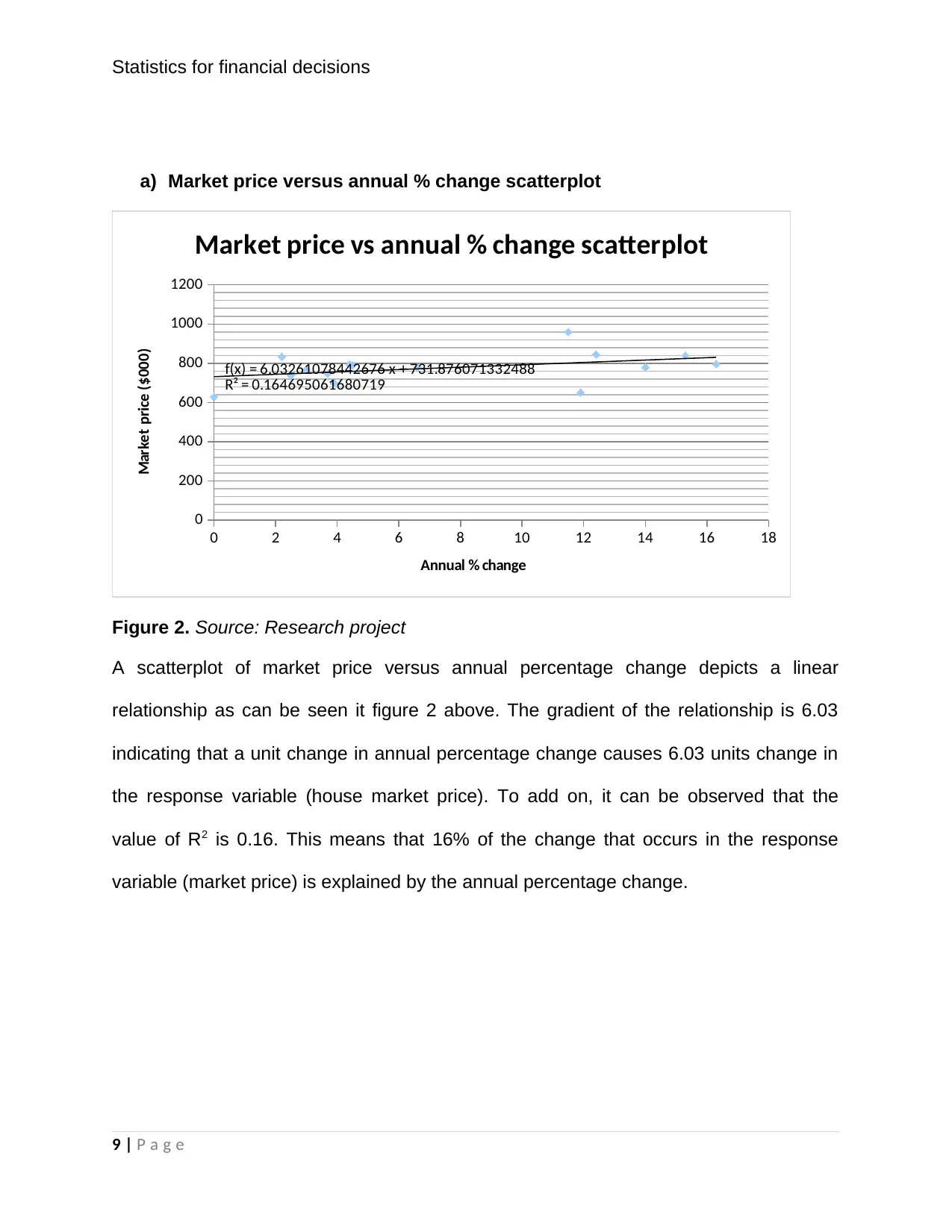
a) Market price versus annual % change scatterplot
0 2 4 6 8 10 12 14 16 18
0
200
400
600
800
1000
1200
f(x) = 6.03261078442676 x + 731.876071332488
R² = 0.164695061680719
Market price vs annual % change scatterplot
Annual % change
Market price ($000)
Figure 2. Source: Research project
A scatterplot of market price versus annual percentage change depicts a linear
relationship as can be seen it figure 2 above. The gradient of the relationship is 6.03
indicating that a unit change in annual percentage change causes 6.03 units change in
the response variable (house market price). To add on, it can be observed that the
value of R2 is 0.16. This means that 16% of the change that occurs in the response
variable (market price) is explained by the annual percentage change.
9 | P a g e
Statistics for financial decisions
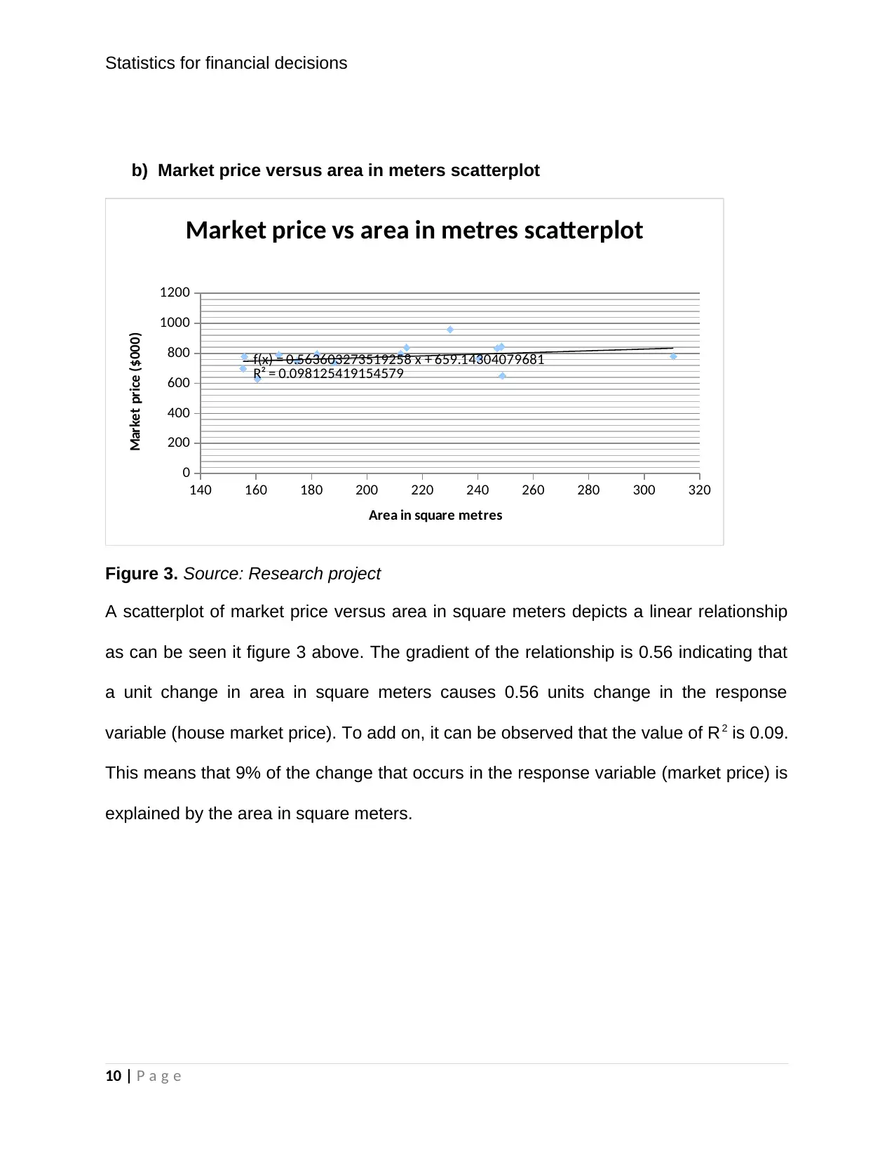
b) Market price versus area in meters scatterplot
140 160 180 200 220 240 260 280 300 320
0
200
400
600
800
1000
1200
f(x) = 0.563603273519258 x + 659.14304079681
R² = 0.098125419154579
Market price vs area in metres scatterplot
Area in square metres
Market price ($000)
Figure 3. Source: Research project
A scatterplot of market price versus area in square meters depicts a linear relationship
as can be seen it figure 3 above. The gradient of the relationship is 0.56 indicating that
a unit change in area in square meters causes 0.56 units change in the response
variable (house market price). To add on, it can be observed that the value of R2 is 0.09.
This means that 9% of the change that occurs in the response variable (market price) is
explained by the area in square meters.
10 | P a g e
Secure Best Marks with AI Grader
Need help grading? Try our AI Grader for instant feedback on your assignments.
Statistics for financial decisions
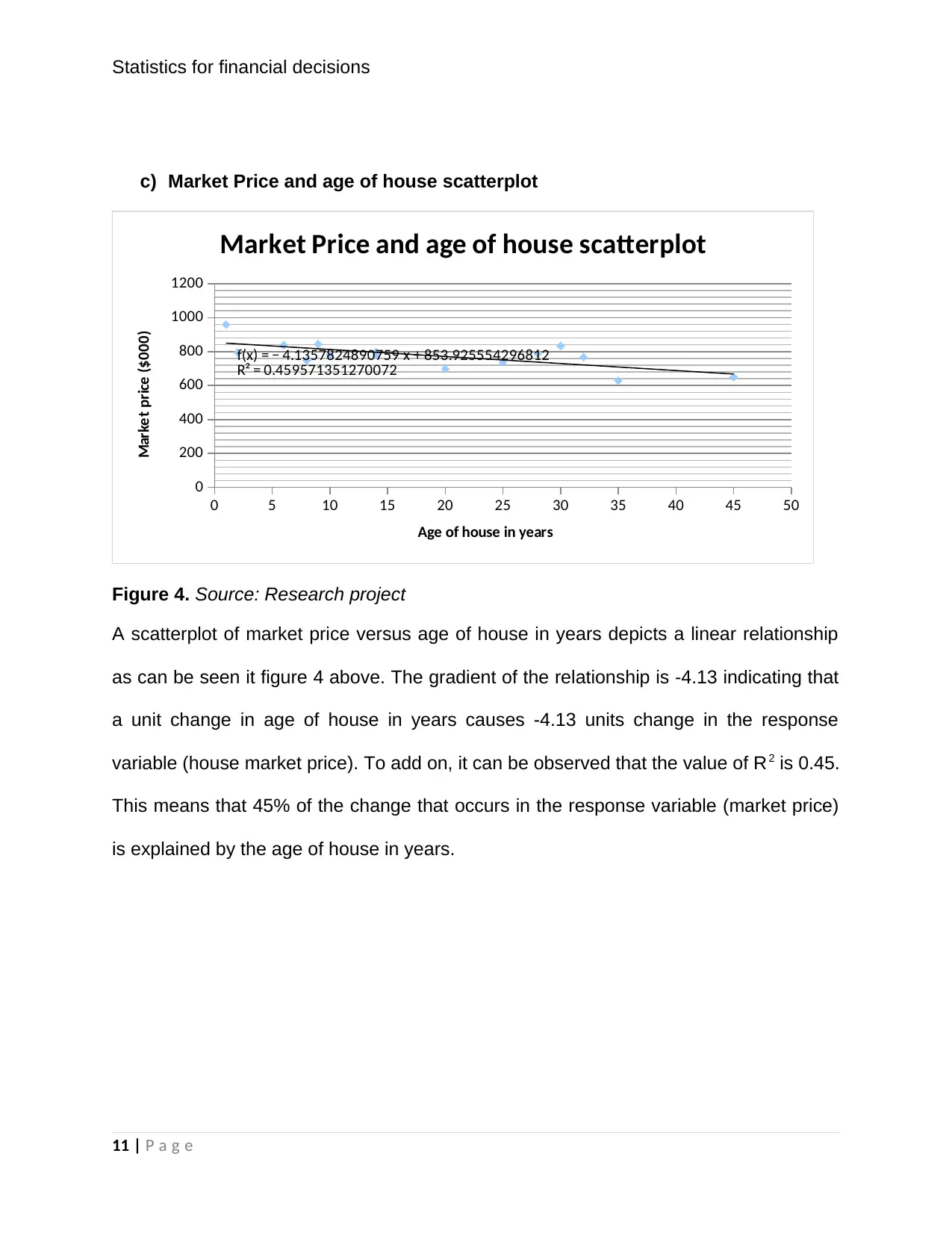
c) Market Price and age of house scatterplot
0 5 10 15 20 25 30 35 40 45 50
0
200
400
600
800
1000
1200
f(x) = − 4.1357824890759 x + 853.925554296812
R² = 0.459571351270072
Market Price and age of house scatterplot
Age of house in years
Market price ($000)
Figure 4. Source: Research project
A scatterplot of market price versus age of house in years depicts a linear relationship
as can be seen it figure 4 above. The gradient of the relationship is -4.13 indicating that
a unit change in age of house in years causes -4.13 units change in the response
variable (house market price). To add on, it can be observed that the value of R2 is 0.45.
This means that 45% of the change that occurs in the response variable (market price)
is explained by the age of house in years.
11 | P a g e
Statistics for financial decisions
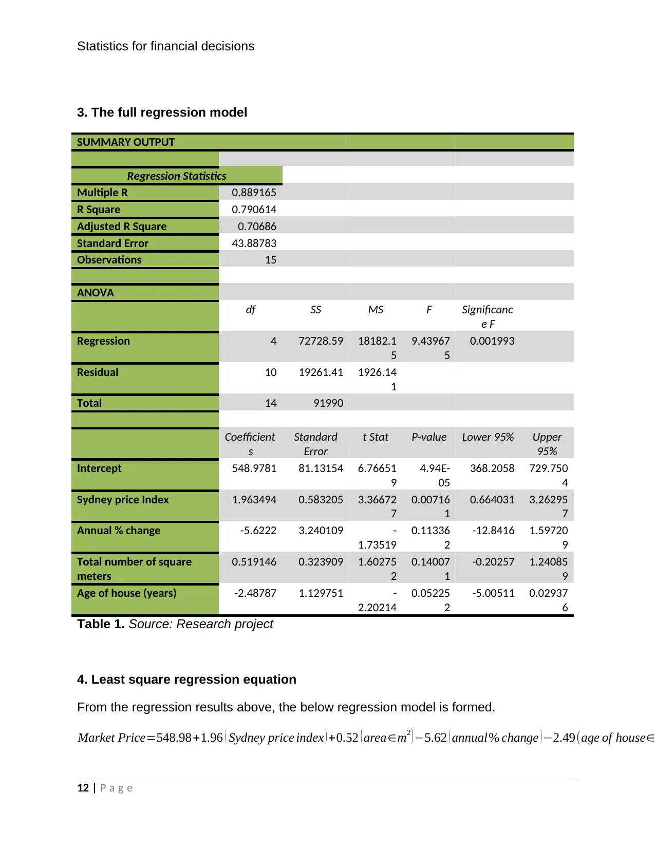
3. The full regression model
SUMMARY OUTPUT
Regression Statistics
Multiple R 0.889165
R Square 0.790614
Adjusted R Square 0.70686
Standard Error 43.88783
Observations 15
ANOVA
df SS MS F Significanc
e F
Regression 4 72728.59 18182.1
5
9.43967
5
0.001993
Residual 10 19261.41 1926.14
1
Total 14 91990
Coefficient
s
Standard
Error
t Stat P-value Lower 95% Upper
95%
Intercept 548.9781 81.13154 6.76651
9
4.94E-
05
368.2058 729.750
4
Sydney price Index 1.963494 0.583205 3.36672
7
0.00716
1
0.664031 3.26295
7
Annual % change -5.6222 3.240109 -
1.73519
0.11336
2
-12.8416 1.59720
9
Total number of square
meters
0.519146 0.323909 1.60275
2
0.14007
1
-0.20257 1.24085
9
Age of house (years) -2.48787 1.129751 -
2.20214
0.05225
2
-5.00511 0.02937
6
Table 1. Source: Research project
4. Least square regression equation
From the regression results above, the below regression model is formed.
Market Price=548.98+1.96 ( Sydney price index ) +0.52 ( area∈m2 ) −5.62 ( annual% change )−2.49(age of house∈
12 | P a g e
Statistics for financial decisions
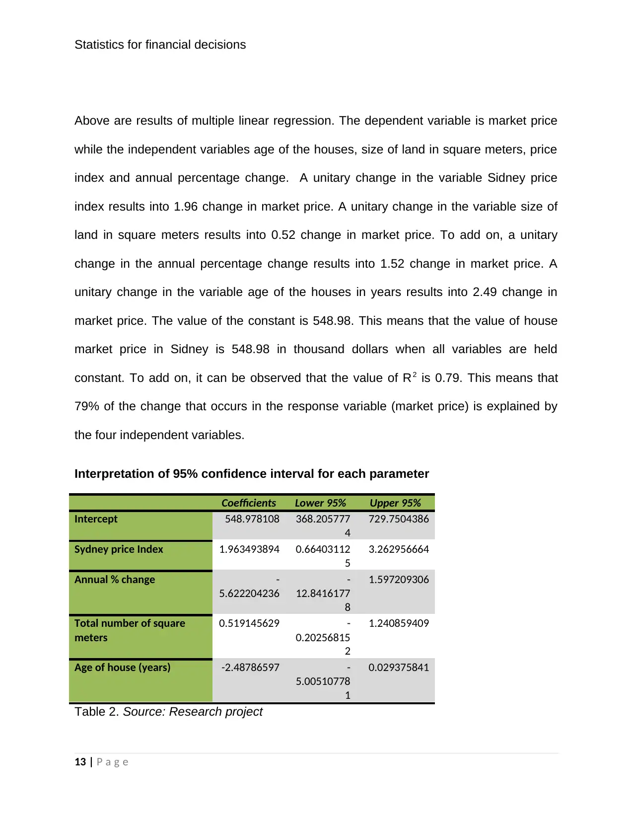
Above are results of multiple linear regression. The dependent variable is market price
while the independent variables age of the houses, size of land in square meters, price
index and annual percentage change. A unitary change in the variable Sidney price
index results into 1.96 change in market price. A unitary change in the variable size of
land in square meters results into 0.52 change in market price. To add on, a unitary
change in the annual percentage change results into 1.52 change in market price. A
unitary change in the variable age of the houses in years results into 2.49 change in
market price. The value of the constant is 548.98. This means that the value of house
market price in Sidney is 548.98 in thousand dollars when all variables are held
constant. To add on, it can be observed that the value of R2 is 0.79. This means that
79% of the change that occurs in the response variable (market price) is explained by
the four independent variables.
Interpretation of 95% confidence interval for each parameter
Coefficients Lower 95% Upper 95%
Intercept 548.978108 368.205777
4
729.7504386
Sydney price Index 1.963493894 0.66403112
5
3.262956664
Annual % change -
5.622204236
-
12.8416177
8
1.597209306
Total number of square
meters
0.519145629 -
0.20256815
2
1.240859409
Age of house (years) -2.48786597 -
5.00510778
1
0.029375841
Table 2. Source: Research project
13 | P a g e
Paraphrase This Document
Need a fresh take? Get an instant paraphrase of this document with our AI Paraphraser
Statistics for financial decisions
The research also sought to establish the limits within which the coefficients lie. A
precision of 95% confidence interval was used. The second and the third column of
table 2 above show where the coefficients will lie 95 times out of 100.
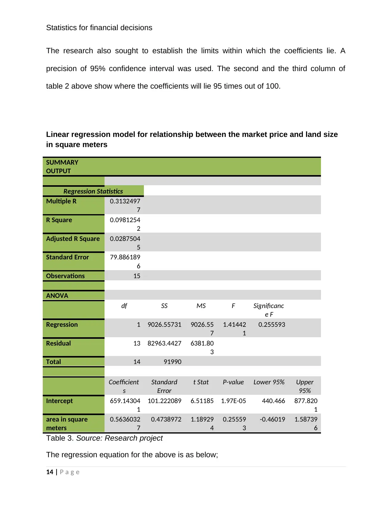
Linear regression model for relationship between the market price and land size
in square meters
SUMMARY
OUTPUT
Regression Statistics
Multiple R 0.3132497
7
R Square 0.0981254
2
Adjusted R Square 0.0287504
5
Standard Error 79.886189
6
Observations 15
ANOVA
df SS MS F Significanc
e F
Regression 1 9026.55731 9026.55
7
1.41442
1
0.255593
Residual 13 82963.4427 6381.80
3
Total 14 91990
Coefficient
s
Standard
Error
t Stat P-value Lower 95% Upper
95%
Intercept 659.14304
1
101.222089 6.51185 1.97E-05 440.466 877.820
1
area in square
meters
0.5636032
7
0.4738972 1.18929
4
0.25559
3
-0.46019 1.58739
6
Table 3. Source: Research project
The regression equation for the above is as below;
14 | P a g e
The research also sought to establish the limits within which the coefficients lie. A
precision of 95% confidence interval was used. The second and the third column of
table 2 above show where the coefficients will lie 95 times out of 100.
Linear regression model for relationship between the market price and land size
in square meters
SUMMARY
OUTPUT
Regression Statistics
Multiple R 0.3132497
7
R Square 0.0981254
2
Adjusted R Square 0.0287504
5
Standard Error 79.886189
6
Observations 15
ANOVA
df SS MS F Significanc
e F
Regression 1 9026.55731 9026.55
7
1.41442
1
0.255593
Residual 13 82963.4427 6381.80
3
Total 14 91990
Coefficient
s
Standard
Error
t Stat P-value Lower 95% Upper
95%
Intercept 659.14304
1
101.222089 6.51185 1.97E-05 440.466 877.820
1
area in square
meters
0.5636032
7
0.4738972 1.18929
4
0.25559
3
-0.46019 1.58739
6
Table 3. Source: Research project
The regression equation for the above is as below;
14 | P a g e
Statistics for financial decisions
Market Price=0.56 ( area∈square meters ) +659.14
The value of R2 is 0.1. This means that 10% of the change that occurs in the response
variable (market price) is explained by the area of land in square meters.
Comparison of the two models
In order to select the best model, we rely on the value of R 2. The higher the value of r-
squared, the better the model. So if we compare the value of R2 which are 0.1 and 0.79,
we choose the model with the r-squared of 0.79 because it is able to explain much of
the variation that occurs in response variable. The models compared are as below.
Market Price=0.56 ( area∈square meters ) +659.14
With R2 value of 0.1
And;
Market Price=548.98+1.96 ( Sydney price index ) +0.52 ( area∈m2 ) −5.62 ( annual% change )−2.49(age of house∈
With R2 value of 0.79
Conclusion
The main objective of this research was to identify the major determinants of prices of
houses in the city of Sidney in Australia. The size of land in square meters, house price
15 | P a g e
Market Price=0.56 ( area∈square meters ) +659.14
The value of R2 is 0.1. This means that 10% of the change that occurs in the response
variable (market price) is explained by the area of land in square meters.
Comparison of the two models
In order to select the best model, we rely on the value of R 2. The higher the value of r-
squared, the better the model. So if we compare the value of R2 which are 0.1 and 0.79,
we choose the model with the r-squared of 0.79 because it is able to explain much of
the variation that occurs in response variable. The models compared are as below.
Market Price=0.56 ( area∈square meters ) +659.14
With R2 value of 0.1
And;
Market Price=548.98+1.96 ( Sydney price index ) +0.52 ( area∈m2 ) −5.62 ( annual% change )−2.49(age of house∈
With R2 value of 0.79
Conclusion
The main objective of this research was to identify the major determinants of prices of
houses in the city of Sidney in Australia. The size of land in square meters, house price
15 | P a g e
Statistics for financial decisions
index, annual price change and age of the house were identified as the major
determinants of the house prices in the city. Various scatterplots have been drawn to
establish the relationship that exists between the dependent variable (house market
price) and independent variables. The independent variable that was found to have the
strongest influence on the house market price was the annual percentage change while
the variable with the least influence was the size of land in meters. The research study
also found that there was a negative relationship between age of house in years and the
house market price. The model that the research study arrived at had r-squared value of
0.79. The model is as below;
Market Price=548.98+1.96 ( Sydney p rice index ) +0.52 ( area∈m2 ) −5.62 ( annual %change ) −2.49(age of house∈
16 | P a g e
Secure Best Marks with AI Grader
Need help grading? Try our AI Grader for instant feedback on your assignments.
Statistics for financial decisions
References
Abelson, P., & Chung, D. (2005). “The Real story of housing prices in Australia from
1970 to 2003”. The Australian Economic Review, 38(3), 265-280.
Dongsheng, C., & Zhong, M. (2010). The bad effects of high housing price on
urbanization of China. Yangtze Forum, 3, 3-7.
Haurin, D. R., & Gill, H. L. (2012). “Effect of income variability on the demand for owner-
occupied housing”. Journal of Urban Economics, 22, 136-150.
Hua, Z. (2008). An analysis of supply and demand curve of real estate market and its
policy implication.. (Vol. 3). Jianghuai Tribune.
Karantonis, A., & Ge, X. J. (2007). “An empirical study of the determinants of Sydney’s
dwelling price”. Pacific Rim Property Research Journal, 13(4), 493-509.
Nellis, J. G. (2011). An empirical analysis of determination of house prices in the United
Kingdom. Urban Studies. (1 ed., Vol. 19).
Quigley , M. J. (2009). Real estate prices and economic cycles. International Estate
Review, 2, 5-8.
Shisong, H., & Hongmei, C. (2009). The mystery of housing price. Beijing: Social
Sciences Academic Press.
17 | P a g e

Statistics for financial decisions
18 | P a g e
18 | P a g e
1 out of 18
Related Documents


Your All-in-One AI-Powered Toolkit for Academic Success.
+13062052269
info@desklib.com
Available 24*7 on WhatsApp / Email
![[object Object]](/_next/static/media/star-bottom.7253800d.svg)
Unlock your academic potential
© 2024 | Zucol Services PVT LTD | All rights reserved.