Hypothesis Testing for Wages and Housing Prices in Sydney
VerifiedAdded on 2023/06/12
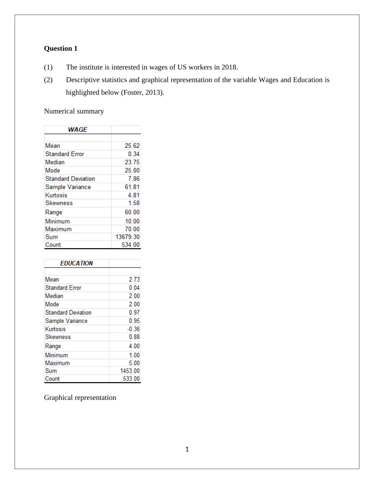
|9
|1266
|287
AI Summary
This article discusses hypothesis testing for wages and housing prices in Sydney. It covers numerical summaries and graphical representations of wages and education levels, and the validity of claims related to proportion and average wage per hour. It also explains how to perform a two independent sample t test for housing prices in two suburbs of Sydney. The article provides insights into statistics for business decision making.
Contribute Materials
Your contribution can guide someone’s learning journey. Share your
documents today.
1 out of 9
Related Documents


Your All-in-One AI-Powered Toolkit for Academic Success.
+13062052269
info@desklib.com
Available 24*7 on WhatsApp / Email
![[object Object]](/_next/static/media/star-bottom.7253800d.svg)
© 2024 | Zucol Services PVT LTD | All rights reserved.