MATLAB Simulink Assignment: Control Systems
VerifiedAdded on  2023/06/14
|20
|1517
|463
AI Summary
This assignment involves solving problems related to control systems using MATLAB Simulink. The topics covered include stabilizing systems, sampling theorem, state space representation, and designing proportional control. The solutions are presented in the form of MATLAB code and simulation results.
Contribute Materials
Your contribution can guide someone’s learning journey. Share your
documents today.
UNIVERSITY AFFILIATION
FACULTY OR DEPARTMENT
COURSE ID & NAME
TITLE:
STUDENT NAME:
STUDENT REGISTRATION NUMBER:
PROFESSOR (TUTOR)
DATE OF SUBMISSION
FACULTY OR DEPARTMENT
COURSE ID & NAME
TITLE:
STUDENT NAME:
STUDENT REGISTRATION NUMBER:
PROFESSOR (TUTOR)
DATE OF SUBMISSION
Secure Best Marks with AI Grader
Need help grading? Try our AI Grader for instant feedback on your assignments.
ASSIGNMENT I
QUESTION 1
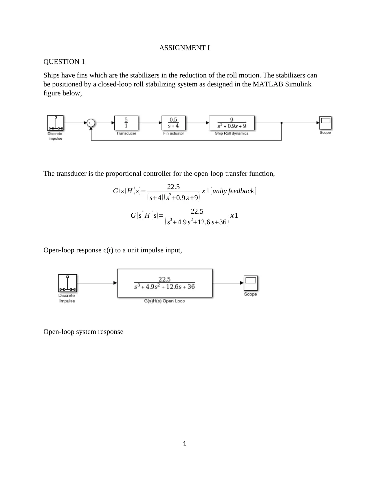
Ships have fins which are the stabilizers in the reduction of the roll motion. The stabilizers can
be positioned by a closed-loop roll stabilizing system as designed in the MATLAB Simulink
figure below,
The transducer is the proportional controller for the open-loop transfer function,
G ( s ) H ( s )= 22.5
( s+ 4 ) ( s2 +0.9 s +9 ) x 1 ( unity feedback )
G ( s ) H ( s ) = 22.5
( s3 + 4.9 s2+12.6 s+36 ) x 1
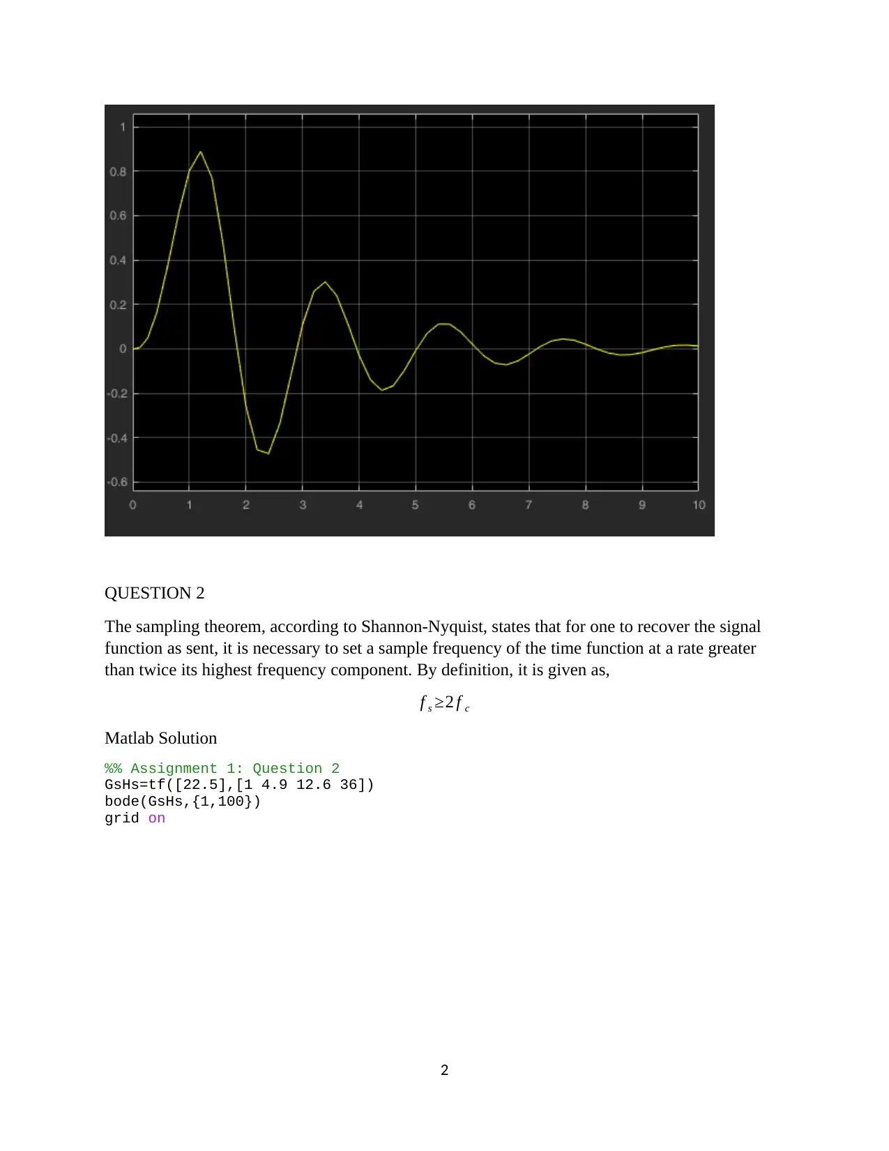
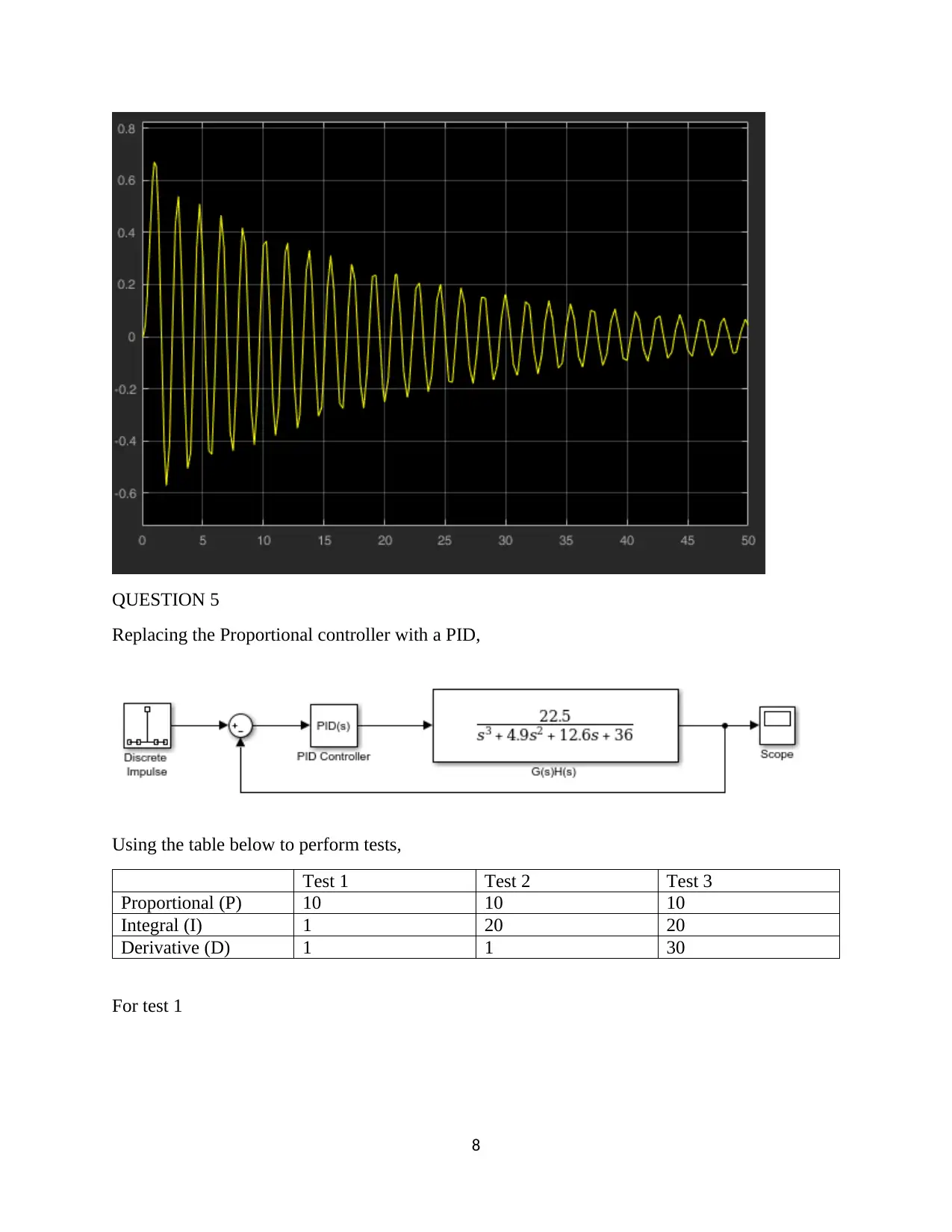
Open-loop response c(t) to a unit impulse input,
Open-loop system response
1
QUESTION 2
The sampling theorem, according to Shannon-Nyquist, states that for one to recover the signal
function as sent, it is necessary to set a sample frequency of the time function at a rate greater
than twice its highest frequency component. By definition, it is given as,
f s ≥2 f c
Matlab Solution
%% Assignment 1: Question 2
GsHs=tf([22.5],[1 4.9 12.6 36])
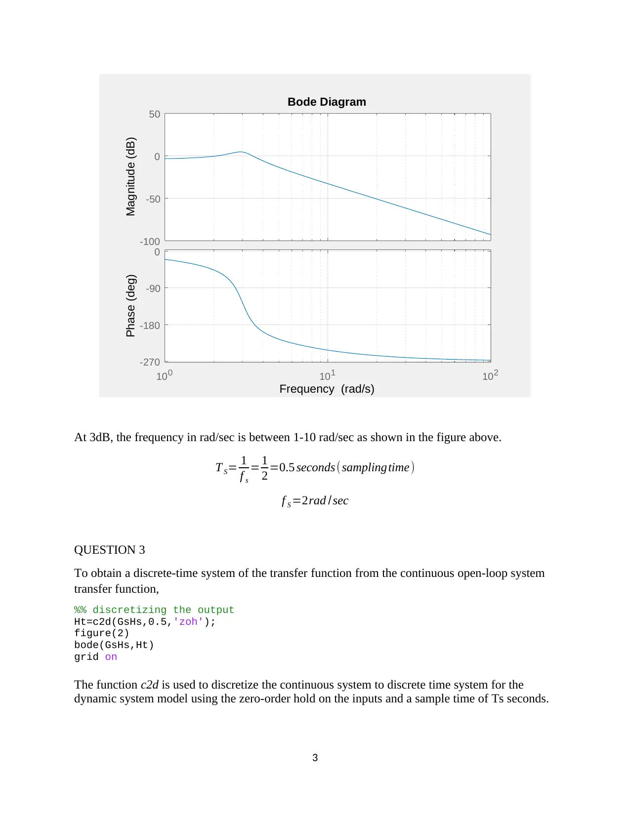
bode(GsHs,{1,100})
grid on
2
-100
-50
0
50
Magnitude (dB)
100 101 102
-270
-180
-90
0
Phase (deg)
Bode Diagram
Frequency (rad/s)
At 3dB, the frequency in rad/sec is between 1-10 rad/sec as shown in the figure above.
T S= 1
f s
= 1
2 =0.5 seconds( samplingtime)
f S =2rad /sec
QUESTION 3
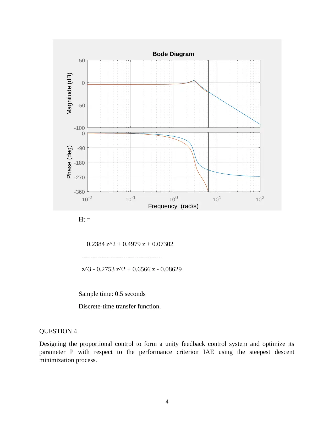
To obtain a discrete-time system of the transfer function from the continuous open-loop system
transfer function,
%% discretizing the output
Ht=c2d(GsHs,0.5,'zoh');
figure(2)
bode(GsHs,Ht)
grid on
The function c2d is used to discretize the continuous system to discrete time system for the
dynamic system model using the zero-order hold on the inputs and a sample time of Ts seconds.
3
Secure Best Marks with AI Grader
Need help grading? Try our AI Grader for instant feedback on your assignments.
-100
-50
0
50
Magnitude (dB)
10-2 10-1 100 101 102
-360
-270
-180
-90
0
Phase (deg)
Bode Diagram
Frequency (rad/s)
Ht =
0.2384 z^2 + 0.4979 z + 0.07302
-------------------------------------
z^3 - 0.2753 z^2 + 0.6566 z - 0.08629
Sample time: 0.5 seconds
Discrete-time transfer function.
QUESTION 4
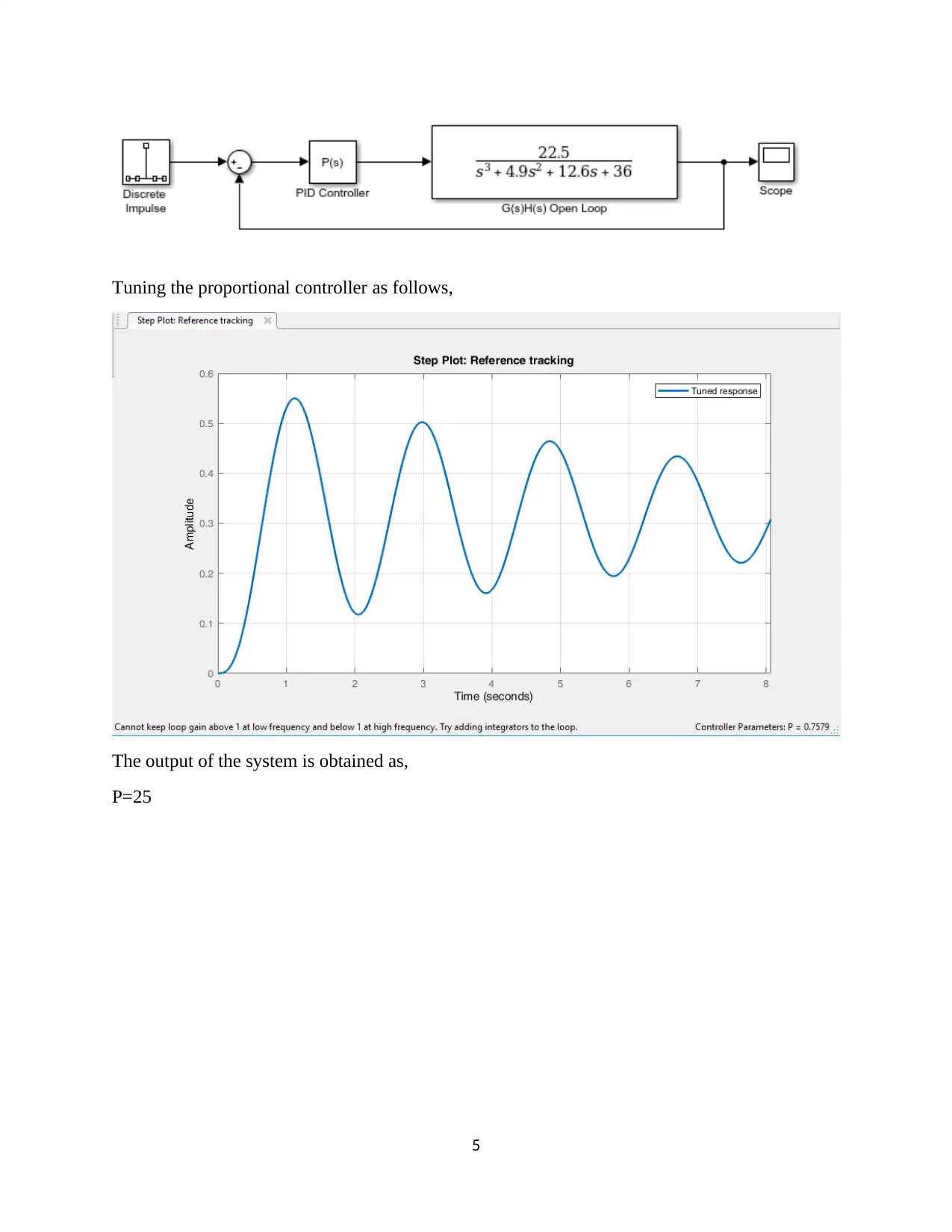
Designing the proportional control to form a unity feedback control system and optimize its
parameter P with respect to the performance criterion IAE using the steepest descent
minimization process.
4
Tuning the proportional controller as follows,
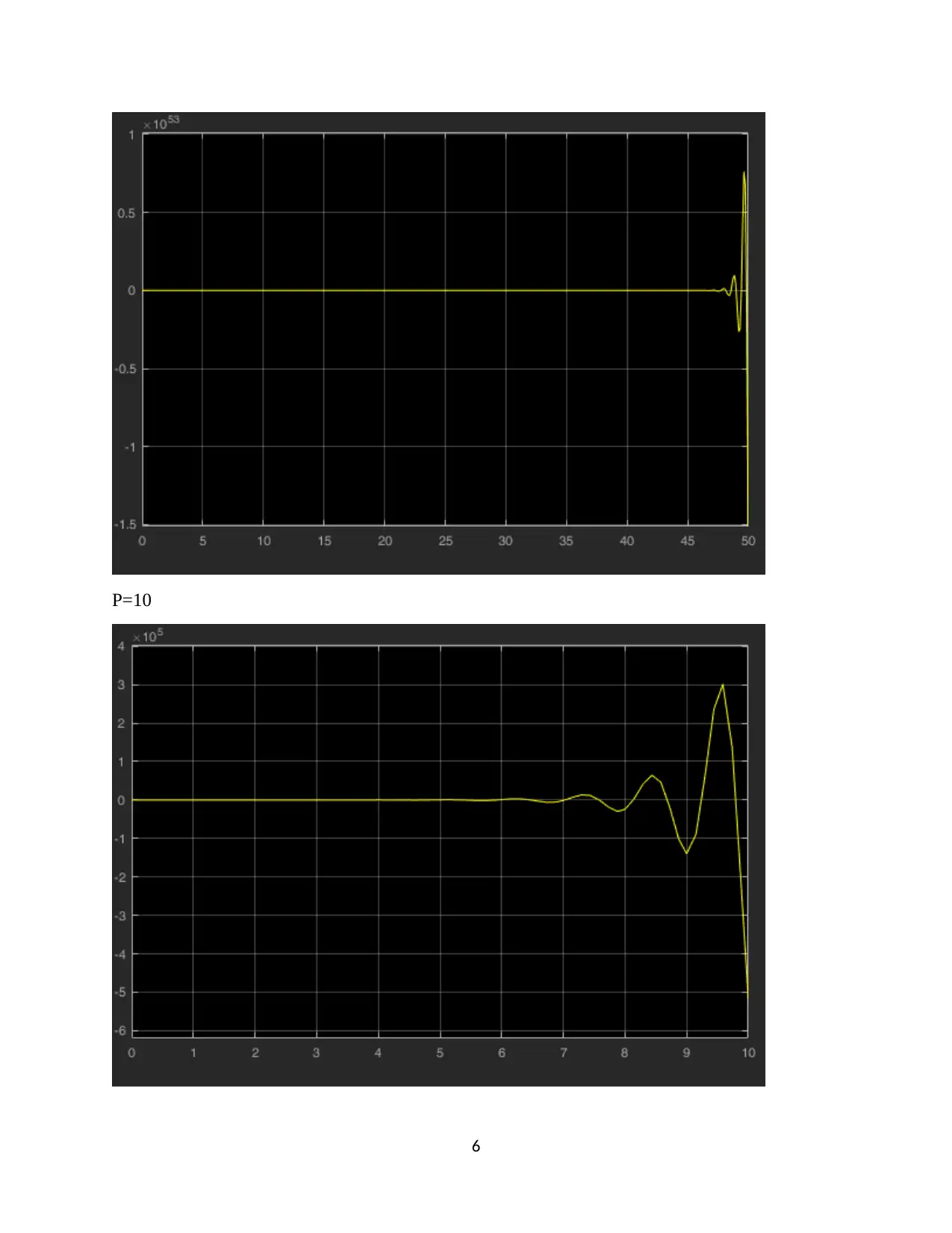
The output of the system is obtained as,
P=25
5
The output of the system is obtained as,
P=25
5
P=10
6
6
Paraphrase This Document
Need a fresh take? Get an instant paraphrase of this document with our AI Paraphraser
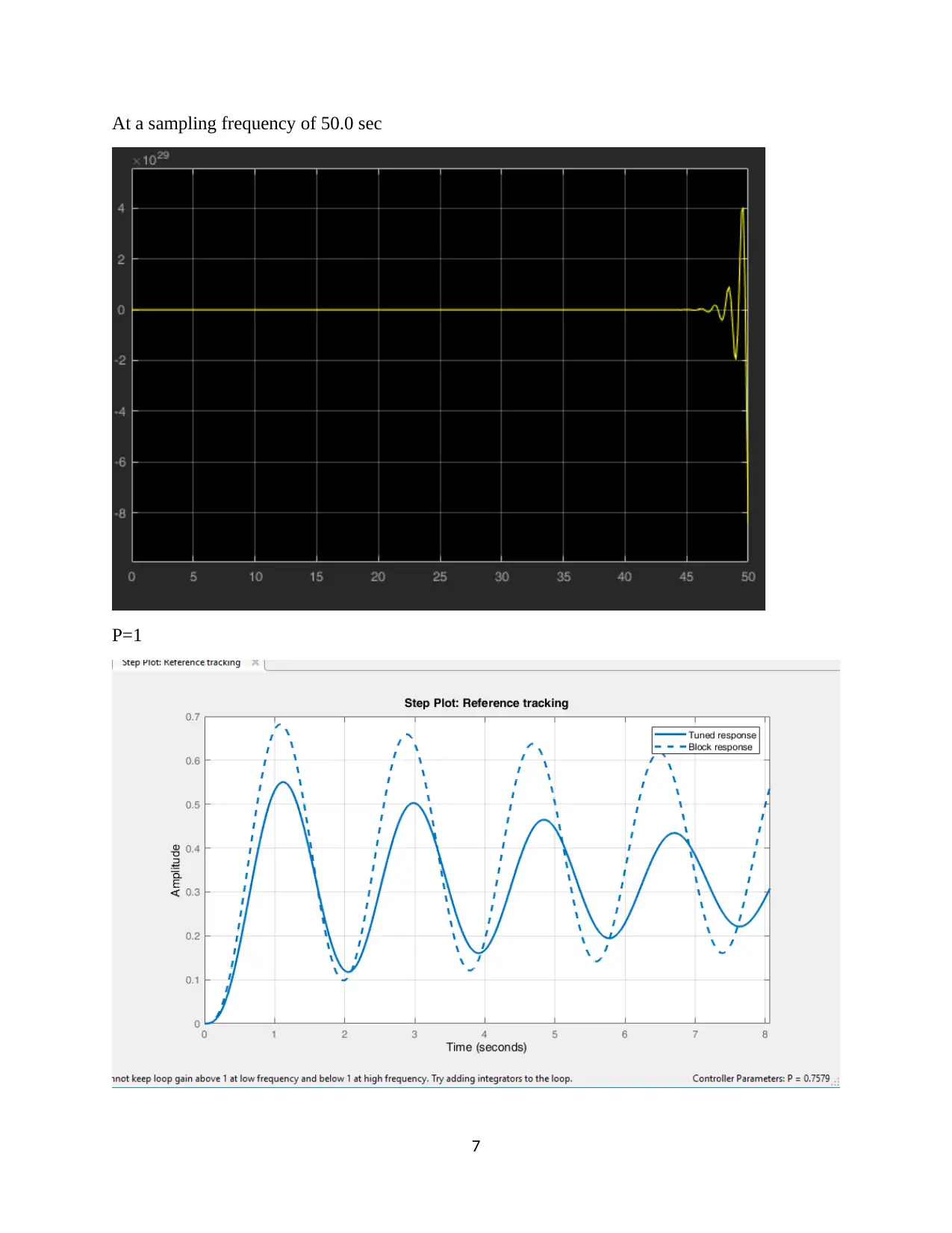
At a sampling frequency of 50.0 sec
P=1
7
P=1
7
QUESTION 5
Replacing the Proportional controller with a PID,
Using the table below to perform tests,
Test 1 Test 2 Test 3
Proportional (P) 10 10 10
Integral (I) 1 20 20
Derivative (D) 1 1 30
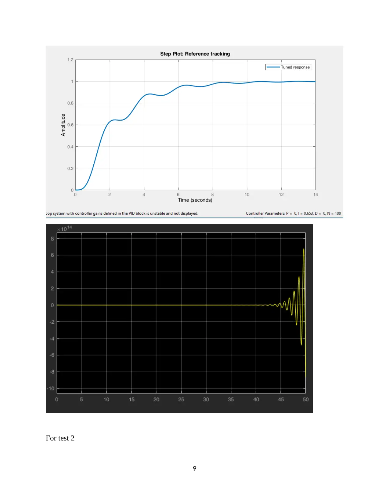
For test 1
8
Replacing the Proportional controller with a PID,
Using the table below to perform tests,
Test 1 Test 2 Test 3
Proportional (P) 10 10 10
Integral (I) 1 20 20
Derivative (D) 1 1 30
For test 1
8
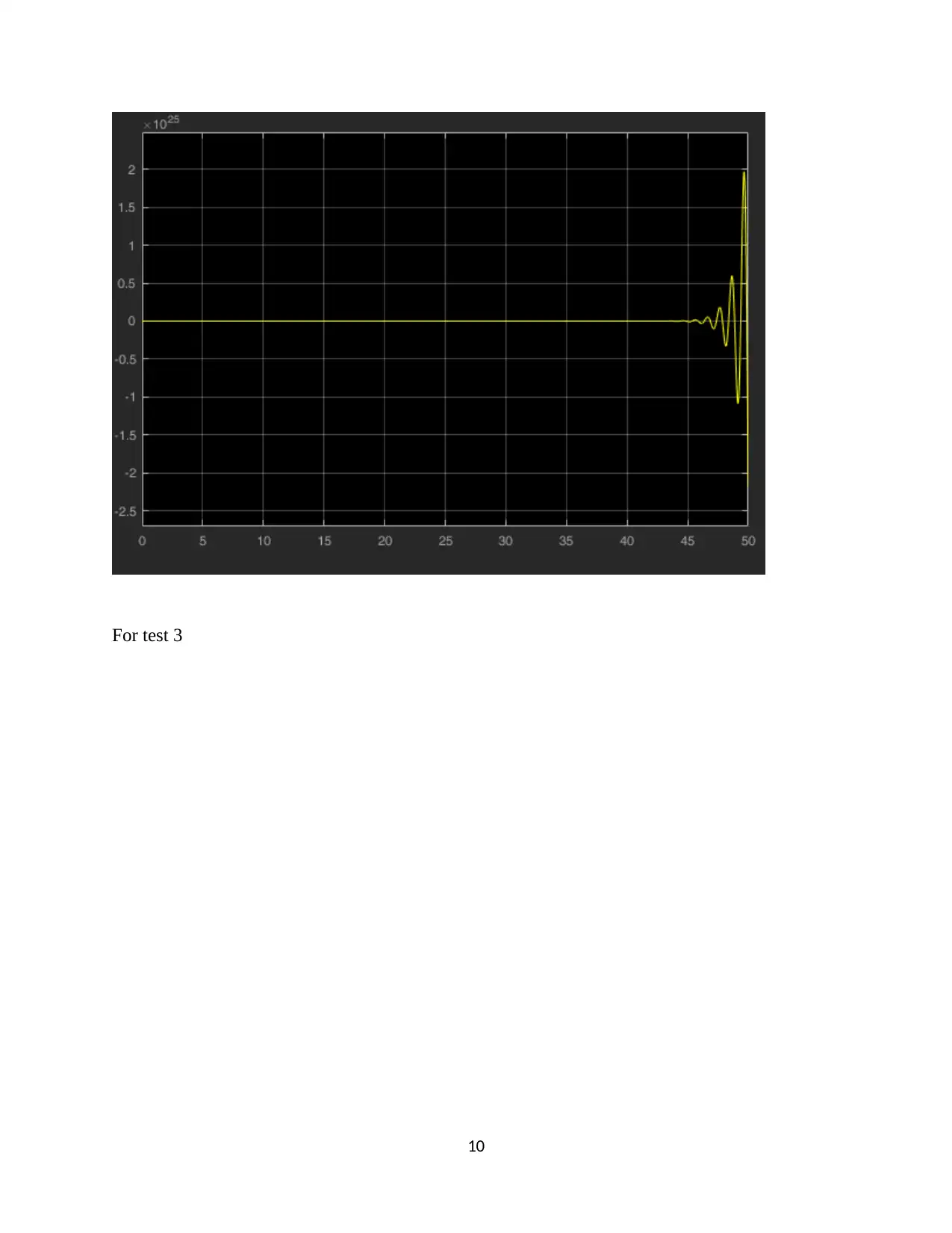
For test 2
9
9
Secure Best Marks with AI Grader
Need help grading? Try our AI Grader for instant feedback on your assignments.
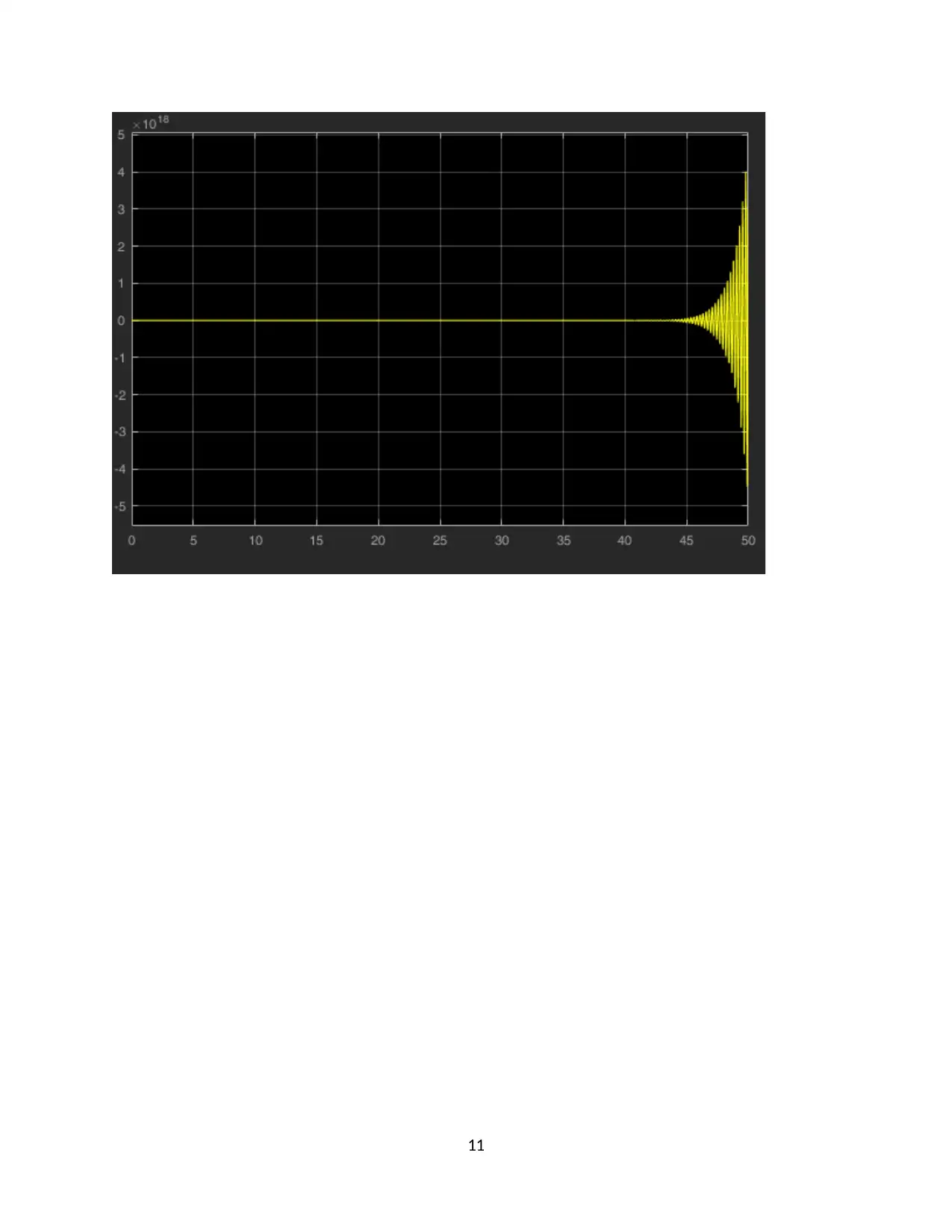
For test 3
10
10
11
ASSIGNMENT 2
QUESTION 1
Block diagram for the position control system with a power amplifier, motor and load, as well as
a converter to the angular velocity. The system is simulated on MATLAB as shown,
clc
close all
format short
p_amp=tf([100],[1 100]); %Power Amplifier TF
m_load=tf([0.2083],[1 1.71 0]); % Motor And Load TF
GsHs2=tf([20.83],[1 101.71 171]) % open loop TF in continuous time
a=20.83;
b=[1 101.71 171];
%% State space form from the continuous time transfer function; It returns
... 4 matrices of the state space representation of the single input TF
[A,B,C,D]=tf2ss(a,b)
The state space canonical form representation,
˙x= Ax+ Bu
y=Cx + Du
˙x= [ −101.71 −171
1 0 ] x+ [ 1
0 ] u
y= [0 20.83 ] x + [ 0 ] u
Therefore,
˙x= [ −272.71
1 ] x +u
y=20.83 x
Using MATLAB to achieve the Output,
clc
close all
format short
p_amp=tf([100],[1 100]); %Power Amplifier TF
m_load=tf([0.2083],[1 1.71 0]); % Motor And Load TF
GsHs2=tf([20.83],[1 101.71 171]) % open loop TF in continuous time
a=20.83;
b=[1 101.71 171];
%% State space form from the continuous time transfer function; It returns
12
Paraphrase This Document
Need a fresh take? Get an instant paraphrase of this document with our AI Paraphraser
... 4 matrices of the state space representation of the single input TF
[A,B,C,D]=tf2ss(a,b)
% alternatively,
sys=ss(GsHs2)
sys.InputDelay(1)
The solution is obtained as
sys =
A =
x1 x2
x1 -101.7 -10.69
x2 16 0
B =
u1
x1 1
x2 0
C =
x1 x2
y1 0 1.302
D =
u1
y1 0
Continuous-time state-space model.
QUESTION 2
Discretizing the system into a discrete time system of the form as shown below,
X ( k +1 )=Φ X ( k )+ Γ u ( k )
y=CX ( k )
Using an input delay of 1
test1 = c2dOptions('Method','tustin','FractDelayApproxOrder',3);
sysd1 = c2d(sys,1,test1)
The output is obtained as
sysd1 =
13
A =
x1 x2
x1 -0.9789 -0.113
x2 0.1691 0.09624
B =
u1
x1 0.01057
x2 0.08456
C =
x1 x2
y1 0.1101 0.7136
D =
u1
y1 0.05504
Sample time: 1 seconds
Discrete-time state-space model.
QUESTION 3
Selecting a proper sampling interval T for the simulation.
%% QUESTION 3: SIMULATING THE DISCRETE TIME SYSTEM - changing T to observe
... the response.
sys2=tf(20.83,[1 101.71 171],'InputDelay',0.3)
sysdiscrete=c2d(sys2,0.5)
The discrete transfer function is obtained as,
sysdiscrete =
0.03378 z^2 + 0.03623 z + 1.858e-12
z^(-1) * -----------------------------------
z^2 - 0.4253 z
Sample time: 0.5 seconds
Discrete-time transfer function.
14
x1 x2
x1 -0.9789 -0.113
x2 0.1691 0.09624
B =
u1
x1 0.01057
x2 0.08456
C =
x1 x2
y1 0.1101 0.7136
D =
u1
y1 0.05504
Sample time: 1 seconds
Discrete-time state-space model.
QUESTION 3
Selecting a proper sampling interval T for the simulation.
%% QUESTION 3: SIMULATING THE DISCRETE TIME SYSTEM - changing T to observe
... the response.
sys2=tf(20.83,[1 101.71 171],'InputDelay',0.3)
sysdiscrete=c2d(sys2,0.5)
The discrete transfer function is obtained as,
sysdiscrete =
0.03378 z^2 + 0.03623 z + 1.858e-12
z^(-1) * -----------------------------------
z^2 - 0.4253 z
Sample time: 0.5 seconds
Discrete-time transfer function.
14
Simulating on MATLAB/Simulink,
... the response.
sys2=tf(20.83,[1 101.71 171],'InputDelay',0.3)
sysdiscrete=c2d(sys2,0.5)
t=0:0.5:50; % Vector of time samples
u=(rem(t,1)>=0.5); % Square Wave values
lsim(sysdiscrete,u,t) %linear simulation
0 5 10 15 20 25 30 35 40 45 50
0
0.1
0.2
0.3
0.4
0.5
0.6
0.7
0.8
0.9
1
Linear Simulation Results
Time (seconds)
Amplitude
Input: In(1)
Time (seconds): 32.5
Amplitude: 0.933
QUESTION 4
State variable feedback regulator for the closed-loop system
15
Secure Best Marks with AI Grader
Need help grading? Try our AI Grader for instant feedback on your assignments.
Using a unit step input
0 5 10 15 20 25 30 35 40 45 50
-0.5
0
0.5
1
1.5
2
2.5
3
3.5 1010STATE VARIABLE FEEDBACK REGULATOR- CLOSED LOOP SYSTEM
Time(seconds) (seconds)
Dynamic Power System Behavior
Getting the root locus of the discrete system as,
16
0 5 10 15 20 25 30 35 40 45 50
-0.5
0
0.5
1
1.5
2
2.5
3
3.5 1010STATE VARIABLE FEEDBACK REGULATOR- CLOSED LOOP SYSTEM
Time(seconds) (seconds)
Dynamic Power System Behavior
Getting the root locus of the discrete system as,
16
-5 -4 -3 -2 -1 0 1
-1.5
-1
-0.5
0
0.5
1
1.5
0.4 /T
0.3 /T
0.5 /T
0.6 /T
0.7 /T
0.8 /T
0.9 /T
1 /T
0.1 /T
0.2 /T
0.3 /T
0.4 /T
0.5 /T
0.6 /T
0.7 /T
0.8 /T
0.9 /T
1 /T
0.1 /T
0.2 /T
0.1
0.2
0.3
0.4
0.5
0.6
0.7
0.8
0.9
Root Locus
Real Axis
Imaginary Axis
QUESTION 5
Design a dead-beat observer to provide state variables for the regulator.
The dead-beat observer is a duplicate of the plant and has the same inputs and differential
equation as the actual plant. There is an anticipation of errors resulting from the plant,
There are three test observer poles with different values,
17
The output is obtained as a stable system,
18
18
Paraphrase This Document
Need a fresh take? Get an instant paraphrase of this document with our AI Paraphraser
0 5 10 15 20 25 30 35 40 45 50
-1
-0.8
-0.6
-0.4
-0.2
0
0.2
0.4
0.6
0.8
1
Linear Simulation Results (with observer)
Time (sec) (seconds)
Dynamic Power System Behavior
Further analysis,
0 0.01 0.02 0.03 0.04 0.05 0.06 0.07 0.08 0.09 0.1
Time (sec)
-1
-0.8
-0.6
-0.4
-0.2
0
0.2
0.4
0.6
0.8
1
h
hest
hdot
hdotest
i
iest
19
-1
-0.8
-0.6
-0.4
-0.2
0
0.2
0.4
0.6
0.8
1
Linear Simulation Results (with observer)
Time (sec) (seconds)
Dynamic Power System Behavior
Further analysis,
0 0.01 0.02 0.03 0.04 0.05 0.06 0.07 0.08 0.09 0.1
Time (sec)
-1
-0.8
-0.6
-0.4
-0.2
0
0.2
0.4
0.6
0.8
1
h
hest
hdot
hdotest
i
iest
19
1 out of 20
Related Documents
Your All-in-One AI-Powered Toolkit for Academic Success.
 +13062052269
info@desklib.com
Available 24*7 on WhatsApp / Email
Unlock your academic potential
© 2024  |  Zucol Services PVT LTD  |  All rights reserved.