Object and Data Modelling
VerifiedAdded on 2022/09/30
|30
|2071
|459
AI Summary
This article discusses the evaluation of the performance of five machine learning models in Weka. It also covers data mining purposes, stages of data mining, and application of data mining. The article includes three datasets: Iris Dataset, Breast Cancer, and Diabetes Dataset. The article also mentions the classification models used for each dataset and their comparison. The subject is Modelling and the course code is 30. The article does not mention any college or university.
Contribute Materials
Your contribution can guide someone’s learning journey. Share your
documents today.
Running Head: MODELLING 1
Object and Data Modelling
Name of Student
School
Object and Data Modelling
Name of Student
School
Secure Best Marks with AI Grader
Need help grading? Try our AI Grader for instant feedback on your assignments.
MODELLING 2
Classification Performance Evaluation (Task 1).
In this part, there will be an evaluation of the performance of five machine learning models in
Weka. Weka is a non-coding machine learning software from Waikato University and it helps
curb most of the troubles that students who are not good in coding do have, like for example, a
mathematical student might want to get insights on the statistical relations that the variables have
and might decide to use statistical software. In any case, the student lacks the coding skills that
are required for example in the platforms such as Python and R then the student an always opt
for non-coding software and in this software we do have Weka and Rapid Minor as the best
examples.
Three datasets are provided in this case and each is, therefore, has to undergo five classification
machine learning models. The models' performances are then supposed to be compared in bid to
get the one that has the top most accuracy in the whole process. The models that have been listed
for comparison include; MultilayerPerceptron, Naive Bayes, decision tree’s J48, RandomForest
and RERTree (Kotthoff, Thornton, Hoos, Hutter & Leyton-Brown, 2019).
1. Iris Dataset
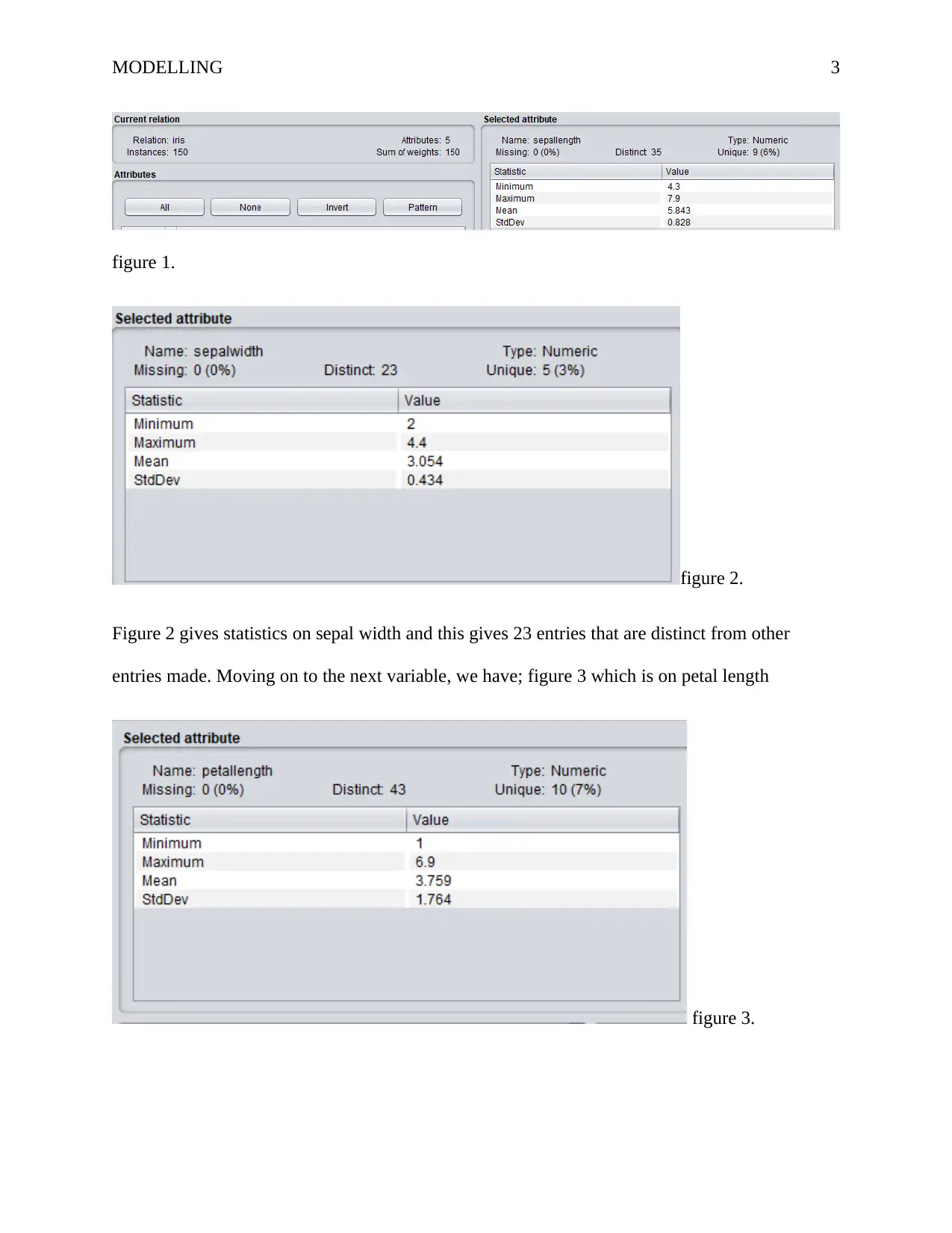
In this case, we will have to begin with the alignment of the Iris dataset and according to the
screen-shot below, we have up to 150 instances as well as 5 number of attributes to be
considered in for analysis. Figure 1 shows the actual descriptive statistics on the sepal length
variable to the right where the mean, standard deviation, the minimum and the maximum
characters are all indicated.
MODELLING 3
figure 1.
figure 2.
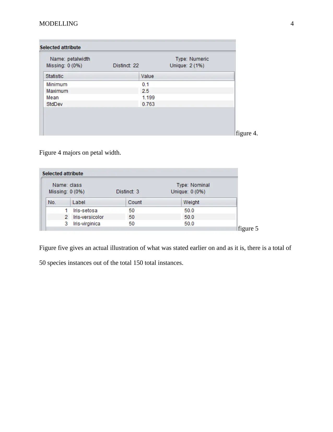
Figure 2 gives statistics on sepal width and this gives 23 entries that are distinct from other
entries made. Moving on to the next variable, we have; figure 3 which is on petal length
figure 3.
figure 1.
figure 2.
Figure 2 gives statistics on sepal width and this gives 23 entries that are distinct from other
entries made. Moving on to the next variable, we have; figure 3 which is on petal length
figure 3.
MODELLING 4
figure 4.
Figure 4 majors on petal width.
figure 5
Figure five gives an actual illustration of what was stated earlier on and as it is, there is a total of
50 species instances out of the total 150 total instances.
figure 4.
Figure 4 majors on petal width.
figure 5
Figure five gives an actual illustration of what was stated earlier on and as it is, there is a total of
50 species instances out of the total 150 total instances.
Secure Best Marks with AI Grader
Need help grading? Try our AI Grader for instant feedback on your assignments.
MODELLING 5
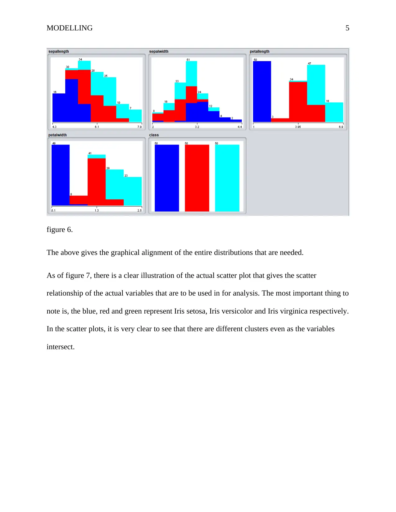
figure 6.
The above gives the graphical alignment of the entire distributions that are needed.
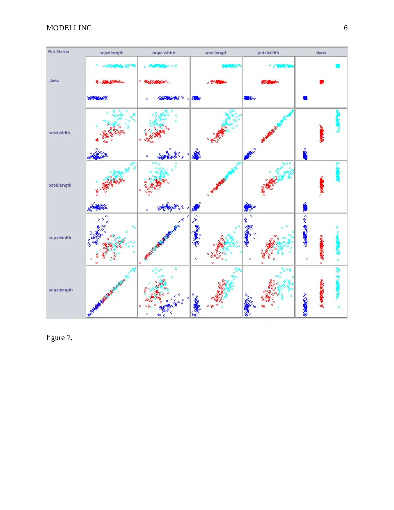
As of figure 7, there is a clear illustration of the actual scatter plot that gives the scatter
relationship of the actual variables that are to be used in for analysis. The most important thing to
note is, the blue, red and green represent Iris setosa, Iris versicolor and Iris virginica respectively.
In the scatter plots, it is very clear to see that there are different clusters even as the variables
intersect.
MODELLING 6
figure 7.
figure 7.
MODELLING 7
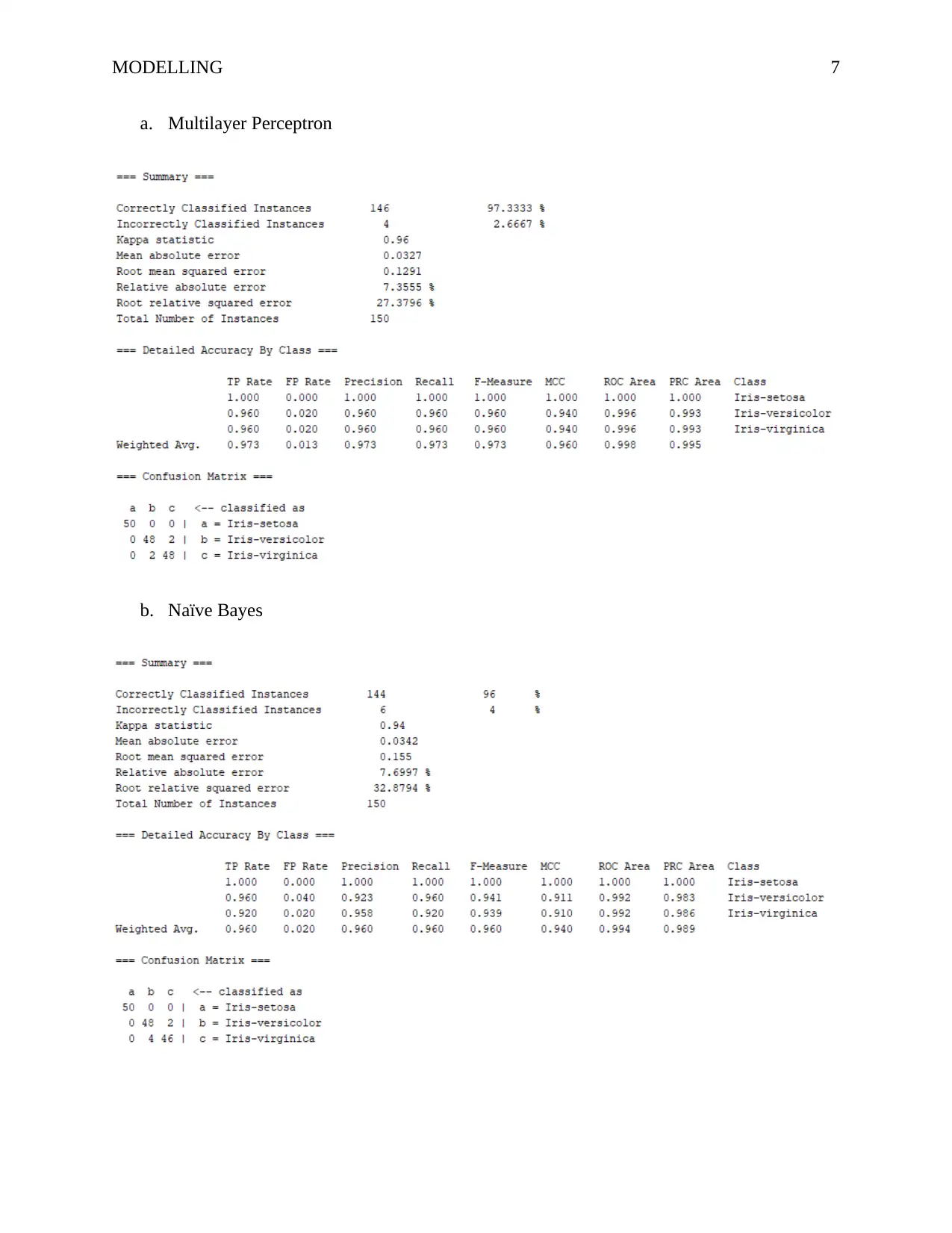
a. Multilayer Perceptron
b. Naïve Bayes
a. Multilayer Perceptron
b. Naïve Bayes
Paraphrase This Document
Need a fresh take? Get an instant paraphrase of this document with our AI Paraphraser
MODELLING 8
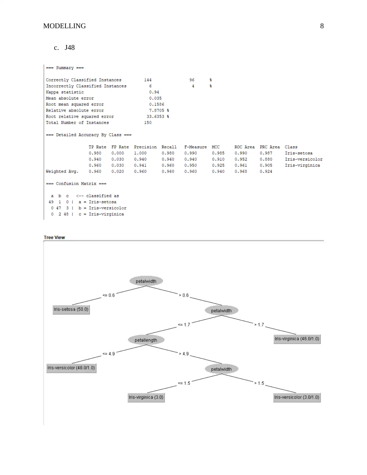
c. J48
c. J48
MODELLING 9
d. Random Forest
e. REP tree
d. Random Forest
e. REP tree
MODELLING 10
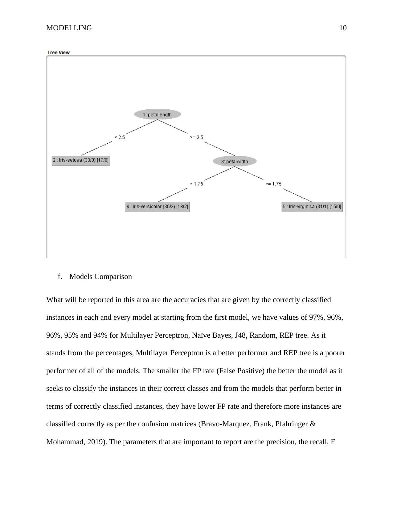
f. Models Comparison
What will be reported in this area are the accuracies that are given by the correctly classified
instances in each and every model at starting from the first model, we have values of 97%, 96%,
96%, 95% and 94% for Multilayer Perceptron, Naïve Bayes, J48, Random, REP tree. As it
stands from the percentages, Multilayer Perceptron is a better performer and REP tree is a poorer
performer of all of the models. The smaller the FP rate (False Positive) the better the model as it
seeks to classify the instances in their correct classes and from the models that perform better in
terms of correctly classified instances, they have lower FP rate and therefore more instances are
classified correctly as per the confusion matrices (Bravo-Marquez, Frank, Pfahringer &
Mohammad, 2019). The parameters that are important to report are the precision, the recall, F
Secure Best Marks with AI Grader
Need help grading? Try our AI Grader for instant feedback on your assignments.
MODELLING 11
measure and the ROC area (Receiver Operator Characteristic) under the curve. The closer these
areas are close to 1 the better the model of classification.
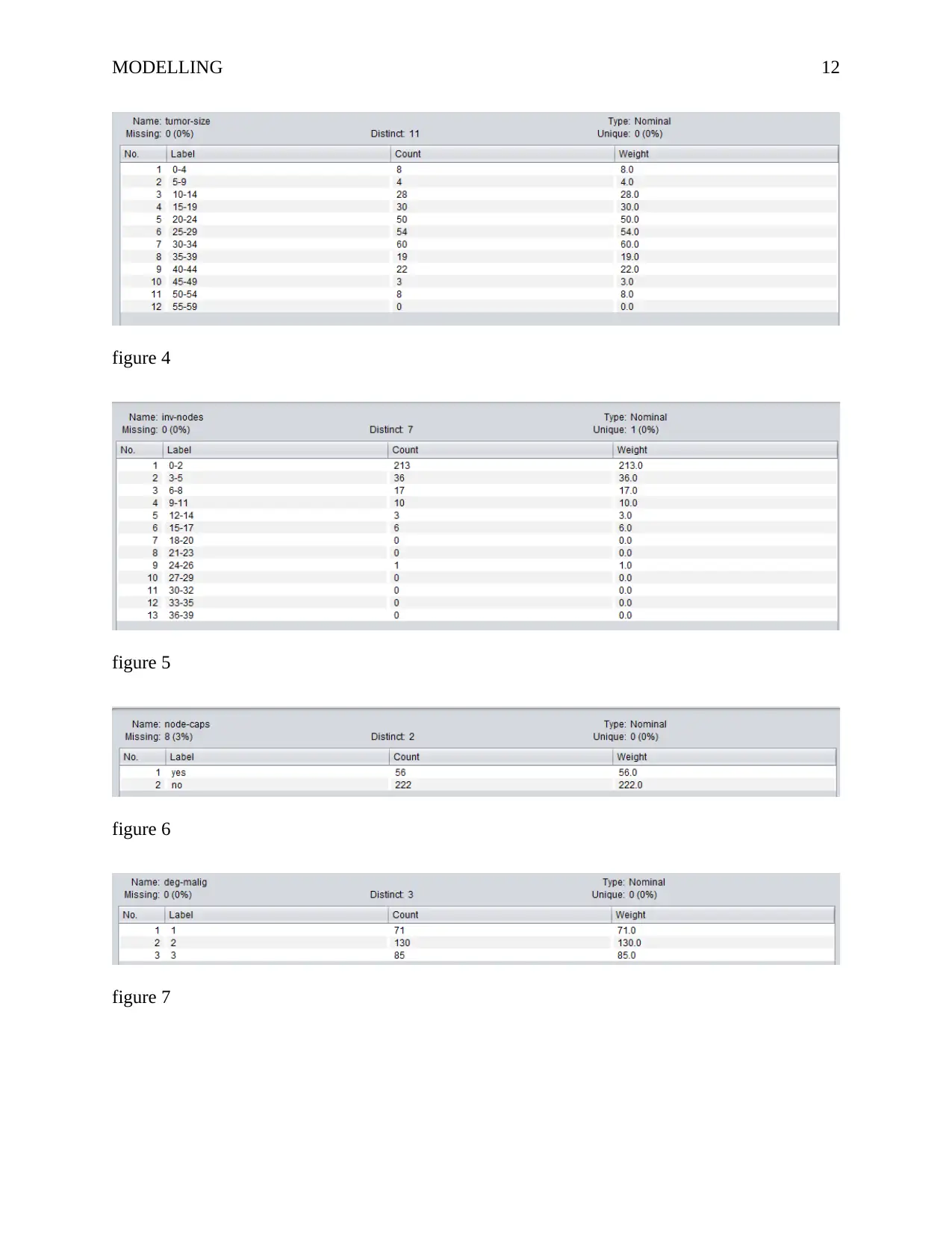
2. Breast Cancer
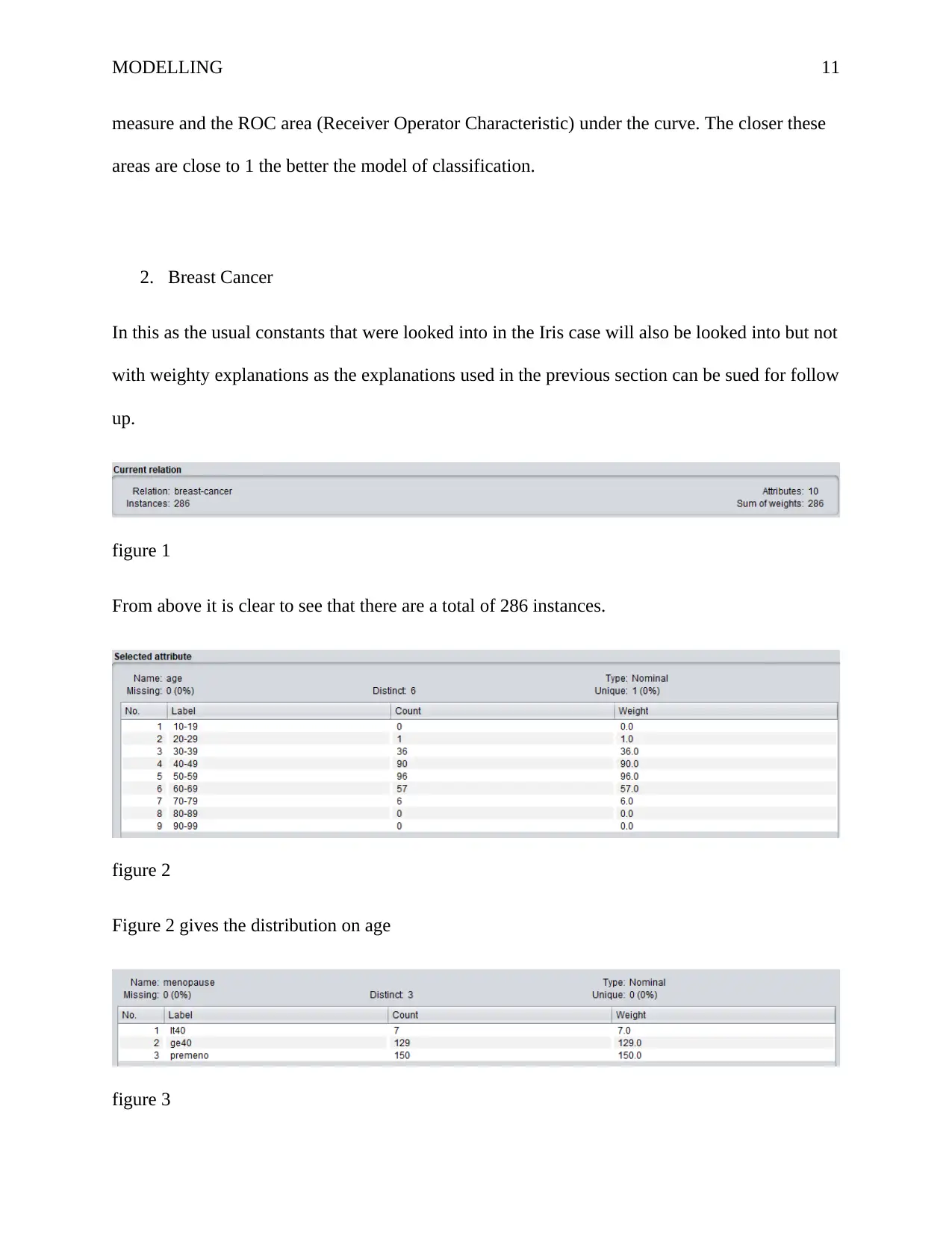
In this as the usual constants that were looked into in the Iris case will also be looked into but not
with weighty explanations as the explanations used in the previous section can be sued for follow
up.
figure 1
From above it is clear to see that there are a total of 286 instances.
figure 2
Figure 2 gives the distribution on age
figure 3
MODELLING 12
figure 4
figure 5
figure 6
figure 7
figure 4
figure 5
figure 6
figure 7
MODELLING 13
figure 8
Figure 9
figure 10
figure 11
figure 8
Figure 9
figure 10
figure 11
Paraphrase This Document
Need a fresh take? Get an instant paraphrase of this document with our AI Paraphraser
MODELLING 14
figure 12.
Figure 12 gives the distribution of all the variables.
figure 12.
Figure 12 gives the distribution of all the variables.
MODELLING 15
1. Classification models
a. Multilayer Perceptron
b. Naïve Bayes
1. Classification models
a. Multilayer Perceptron
b. Naïve Bayes
MODELLING 16
c. J48
c. J48
Secure Best Marks with AI Grader
Need help grading? Try our AI Grader for instant feedback on your assignments.
MODELLING 17
d. Random Forest
d. Random Forest
MODELLING 18
e. REP Tree
e. REP Tree
MODELLING 19
For Multilayer Perceptron, Naïve Bayes, J48, Random and REP tree we have 64%, 71%, 75%,
69% and 70%. As it stands we have that the best performer is Naïve Bayes according to this
dataset.
For Multilayer Perceptron, Naïve Bayes, J48, Random and REP tree we have 64%, 71%, 75%,
69% and 70%. As it stands we have that the best performer is Naïve Bayes according to this
dataset.
Paraphrase This Document
Need a fresh take? Get an instant paraphrase of this document with our AI Paraphraser
MODELLING 20
2. Diabetes Dataset
Figure 1.
Figure 1 shows the graphical distribution of all the variables that there are in the diabetes dataset.
2. Diabetes Dataset
Figure 1.
Figure 1 shows the graphical distribution of all the variables that there are in the diabetes dataset.
MODELLING 21
Figure 2.
From above it is very clear that the points are spread any-how and that there is no clear one place
clustering from the intersection of most variables.
Figure 2.
From above it is very clear that the points are spread any-how and that there is no clear one place
clustering from the intersection of most variables.
MODELLING 22
Classification Models
a. Multilayer Perception
b. Naïve Bayes
Classification Models
a. Multilayer Perception
b. Naïve Bayes
Secure Best Marks with AI Grader
Need help grading? Try our AI Grader for instant feedback on your assignments.
MODELLING 23
c. J48
c. J48
MODELLING 24
d. Random Forest
d. Random Forest
MODELLING 25
e. REP Tree
e. REP Tree
Paraphrase This Document
Need a fresh take? Get an instant paraphrase of this document with our AI Paraphraser
MODELLING 26
From the above dataset, it is very clear that the percentages for the correctly classified instances
are; 75%, 76%, 73%, 75% and 75%. What this gives is that the best performing model for the
classification of the diabetes dataset is Naïve Bayes and the least performing model is J48.
Data Mining Applications (Task 2)
In simple term, data mining, from the word mining, is retrieving data from a specific source for
analysis and better interpretation to aid in getting better results. Scientifically though, data
mining is the statistical processes of finding the anomalies, patterns and the correlation with
large data sets as this helps in predictions of different outcomes that aid in different ways. With
technological advancement, data mining is used in different industries and for different purposes.
MODELLING 27
a. Data Mining Purposes
The obvious purposes as to the use of data mining include; aims of increasing the revenues
earned, help improve customers' relationships amongst themselves as well as with the company
in question, reduce risks and fraudulent activities. Several parameters are used in data mining
and they include, clustering, forecasting, sequence analysis and classification (Zhu, Imamura,
Nikovski & Keogh, 2019). What sequence analysis seeks to find out is what the actual path of
the occurrence of behaviour amongst customers and an undesirable business process is. In
clustering, the groups of patterns are sort for and documented in a way that aggregates them as
they are similar. Classification looks for a new pattern and therefore sets new trends and can
therefore even make the way things are done in an organization to entirely change. Forecasting,
on the other hand, seeks to give a clear prediction of what is expected for the future. What this
means is there can be a forecast on the amount of production expected to be put out the following
production period and finally this can lead to the forecasting of the next period's profits (Feng,
Barbosa & Torres, 2016).
b. Stages of Data Mining
In all of that, one must note that data mining is not a one stage process and that there are up to a
total of four stages. The first stage is the data sources stage and there is the identification of the
database system from where data is to be retrieved from. Data exploration or gathering stage
(second stage) is the actual act of getting the dataset and then exploring it and setting in in a
format that can be used in a way that can better aid easier analysis and algorithms build-up for
company processes. The modelling stage is the third stage and in this stage, the analysis models
are build up but not only analysis models but machine learning models that aid in classification,
regression as well as clustering. The models once built; it can be deployed at the deployment
MODELLING 28
stage which is the last. The deployment stage cannot be reached without testing the model to find
out if it is the best fit model that needs deployment. If a model does not meet the criteria that are
expected of it to meet, then it definitely can be revised and improved before deployment or better
yet, a new model can be built. The only challenge that there is in data mining, development and
the deployment of algorithms is the fact that these algorithms become irrelevant over a short time
and must be changed or improved from time to time.
c. Application of Data Mining
The areas that get the full version of data mining that will be focused on in this report will be,
increase of revenues and customer relations. Take for instance a mobile company, more so a
telecommunication company (Lu, Hongjun, Rudy and Huan, 2017). There are more players and
more customers that do get on board in the long run to offer the same services and this occurs
frequently. What this means is that they actually might pause a competition and are feared
because they might come in offering lower rates in tariffs and better customer concentration.
When this happens the existent firm or firm might get to weep as it will lose profits. To get to
tame customers and make them stay put because it is cheaper to maintain and existent customer
than to acquire new ones. Therefore, this is the stage where data mining stages come to play and
a model is built to get to predict those customers that might leave or rather churn from those that
are loyal. After that, the proactive measures can be taken as per the management of the
organization to help aid save the loss of potential customers. The models that can be used in such
an as are like, linear regression, logistic regression, decision trees and the testing can be done by
the use of ROC, AUC and the confusion matrix (Zheng, 2015).
Secure Best Marks with AI Grader
Need help grading? Try our AI Grader for instant feedback on your assignments.
MODELLING 29
References
Bravo-Marquez, F., Frank, E., Pfahringer, B., & Mohammad, S. M. (2019). AffectiveTweets: a
Weka package for analyzing effect in tweets.
Dua, S., & Du, X. (2016). Data mining and machine learning in cybersecurity. Auerbach
Publications.
Feng, J., Barbosa, L. D. A., & Torres, V. (2016). U.S. Patent No. 9,262,517. Washington, DC:
U.S. Patent and Trademark Office.
Kotthoff, L., Thornton, C., Hoos, H. H., Hutter, F., & Leyton-Brown, K. (2019). Auto-WEKA:
Automatic Model Selection and Hyperparameter Optimization in. Anteil EPB, 81.
Lu, Hongjun, Rudy Setiono, and Huan Liu. "Neurorule: A connectionist approach to data
mining." arXiv preprint arXiv:1701.01358 (2017).
Zheng, Y. (2015). Trajectory data mining: an overview. ACM Transactions on Intelligent
Systems and Technology (TIST), 6(3), p.29.
Zhu, Y., Imamura, M., Nikovski, D., & Keogh, E. (2019). Introducing time series chains: a new
primitive for time series data mining. Knowledge and Information Systems, 60(2), 1135-
1161.
MODELLING 30
1 out of 30
Your All-in-One AI-Powered Toolkit for Academic Success.
+13062052269
info@desklib.com
Available 24*7 on WhatsApp / Email
Unlock your academic potential
© 2024 | Zucol Services PVT LTD | All rights reserved.