Numerical Solutions of PDE | Assignment
Added on 2022-09-07
12 Pages2653 Words103 Views
NUMERICAL SOLUTIONS OF PDE
Problem 1.a)
There various finite difference methods of solving partial differential
equations. The method used depends on the structure and complexity of the
equation of concern. The Partial Differential Equation (PDEs) of interest does
not have an analytical solution and therefore, a numerical method have to be
used to find an approximate solution. The approximation is done at discrete
values of independent variables using an approximation scheme
implemented via a program. An approximated solution is obtained after
manipulation and creation of a finite difference schemes:
Taylor’s Theorem.
This method operates by replacing the over regions of defined independence
variables by points of approximated dependent variables. The partial
derivatives are thereafter estimated from the neighboring values.
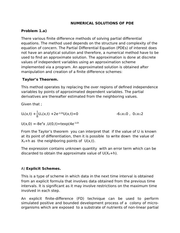
Given that ;
Ut(x,t) + 1
8 Ux(x,t) +2e-1/2tU(x,t)=0 -6≤x≤0 , 0≤x≤2
U(x,0) =-8e4x ,U(0,t)=texp(4e-1/2t
From the Taylor’s theorem you can interpret that if the value of U is known
at its point of differentiation, then it is possible to write down the value of
X0+h as the neighboring points of U(x,t).
The expression contains unknown quantity with an error term which can be
discarded to obtain the approximate value of U(X0+h).
A) Explicit Schemes.
This is a type of scheme in which data in the next time interval is obtained
from an explicit formula that involves data obtained from the previous time
intervals. It is significant as it may involve restrictions on the maximum time
involved in each step.
An explicit finite-difference (FD) technique can be used to perform
simulated positive and bounded development process of a colony of micro-
organisms which are exposed to a substrate of nutrients of non-linear partial
Problem 1.a)
There various finite difference methods of solving partial differential
equations. The method used depends on the structure and complexity of the
equation of concern. The Partial Differential Equation (PDEs) of interest does
not have an analytical solution and therefore, a numerical method have to be
used to find an approximate solution. The approximation is done at discrete
values of independent variables using an approximation scheme
implemented via a program. An approximated solution is obtained after
manipulation and creation of a finite difference schemes:
Taylor’s Theorem.
This method operates by replacing the over regions of defined independence
variables by points of approximated dependent variables. The partial
derivatives are thereafter estimated from the neighboring values.
Given that ;
Ut(x,t) + 1
8 Ux(x,t) +2e-1/2tU(x,t)=0 -6≤x≤0 , 0≤x≤2
U(x,0) =-8e4x ,U(0,t)=texp(4e-1/2t
From the Taylor’s theorem you can interpret that if the value of U is known
at its point of differentiation, then it is possible to write down the value of
X0+h as the neighboring points of U(x,t).
The expression contains unknown quantity with an error term which can be
discarded to obtain the approximate value of U(X0+h).
A) Explicit Schemes.
This is a type of scheme in which data in the next time interval is obtained
from an explicit formula that involves data obtained from the previous time
intervals. It is significant as it may involve restrictions on the maximum time
involved in each step.
An explicit finite-difference (FD) technique can be used to perform
simulated positive and bounded development process of a colony of micro-
organisms which are exposed to a substrate of nutrients of non-linear partial
differential equations The finite difference is specifically modeled in such a
form that it eliminates the parabolic terms in the initial PDE into numerical
sets of linear algebraic equations that can easily be solved. Which ensuring
that the solution remains stable and unbounded. This can be realized from a
model of interconnected estimations fo a diffusion response and functions of
both time and spatial variations as well as the control time-step of
generating a criteria of theoretical stability. An elaborate analysis of
theoretical stability is performed to help realize that our technique is indeed
optimal. The numerical solutions are to be ensured to be non-negative and
bounded.
Consistency: You can conclude that a nominal finite difference scheme is
consistent when it converges to the PDEs we are trying to solve as the space
and time approaches zero. Consistency does not prove relevant when it is
spatial and time discretization are parted. However, a further check is
important at mixed discretization.
Stability: You can only say a finite difference is stable when the difference
between the numerical value solution and the exact value solution are
bounded as it approaches to infinite.
B)Implicit Schemes.
A type of scheme in which data obtained from the next time level happens
on both sides of the difference schemes that involve solving a system of
linear equations .This is characterized by non-stable restrictions. The
maximum time allowed in each step may be much longer than that of the
explicit scheme for the same problem.
A type of Scheme are chosen depending on the accuracy level in need.
Convergence: You can say that a finite difference scheme converges when
its numerical value tends to zero as the space and time discretization also
tend to zero.
Implicit solutions relate only to the simplest systems of equations. Implicit solutions are
not conditionally stable. This can be realized fro mathematical models of the dynamic
problems such as the fluid dynamics.
The stability of the finite difference scheme corresponds to the spread of waves of
information into a solution. Elastic and fluctuating waves may lead to a balance between
inertia and gravity. Kinematic waves is a consequence of the the balance between
resistance and gravity.
1.The problems will be continuously be unstable at the tiny level when the waves move
at higher speed as compared to the dynamic waves. This can however make both
conditions of implicit and explicit schemes to be unstable.
2.As you will often realize that numerical stability is not constant but varies with relative
measures of control of a chosen analysis. This may initiate a hyper volume of higher
dimensions in regard to the locality of the finite volume over lifespan which can emerge
into a courant Number.Courant is the distance travelled over an element’s lifespan .
3. In extension of the initial conditions and in comparison to the current situation,
boundary conditions can be seen as a relatively a time-wise expansion.Therefore,the
space wise direction in which equations are solved becomes significant.
4.Explicit solutions are discriminative, that is, the solutions for each explicit function
within a cell are only meant for that cell. This is not the case with implicit function as any
solution from any cell can be used in any other different cell. AS a result, it is only
applicable in stability for courant numbers<1
5.The solutions for implicit functions are generally stable for even Courant Numbers
greater than 1 when solved simultaneously over a range of cells. For cases of low
courant numbers ,the implicit equations appear top be unstable and are solved in the
wrong direction from the boundaries.
6.Stability of finite difference scheme of PDE cannot guarantee accuracy
level.However,the its accuracy may dependent variable on a balance of influence
between the initial conditions and the boundary mark. As a result,courant
number=1,where both implicit and explicit schemes are most accurate.
7. There always a search of the scheme with the best performance in both the explicit
and implicit schemes as there are several courant numbers with different wave types
and spatial dimensions.However,implicit solutions are much more preferred as
compared to the explicit solutions. Explicit solutions can be coded to run at a higher
pace in relation to the explicit solutions.
You will confirm that the explicit formulation requires values from other loci on the
previous instantaneous time to produce the values of the current loci. This is repetitive
and may but not cumbersome to get involved as the method is very simple and
clear.However,the time step must be maintained to a smaller value to ensure an
accurate stability is met and maintained. This may need many iterations to significantly
calculate time. The explicit formulation needs the values from other nodes at a previous
instant of time to determine the node value of the present one, the computational
calculation method is very simple. However, the time step has to be really small in order
to maintain the stability of this approach, so it will require a huge number of iterations
that could increase significantly the calculation time.
The implicit formulation is more advantageous in solving a defined problem. It may
require much less time as it does not need to verify the stability criterion of each time
step. The manipulation of node values and figures at the current time, relies on the
neighboring figures of every locus at constant period. The equation formation is done
simultaneously.
Implicit schemes are very expensive as compared to explicit formulation. Implicit
schemes and techniques may be unconditionally stable considering each time step and
the problem under specification. Implicit method can use several time steps and get an
exact solution within a short time. Hence it is more reliable as compared to explicit
schemes. This is due to low computer costs and a significant accuracy level.
The disadvantage of the explicit schemes is their conditional stability. Each addition of
the explicit time integration is much less is expensive than the time integration for the
implicit manipulations.
The decision on the explicit and implicit schemes depends on the type and size of the
problem.
Problem 1.b)
Krank-Nicolson Scheme.
This is an implicit scheme in which a partial derivative are approximated at
the time interval n.There is realization of value change between time interval
n and n+1 time interval level.From the resultit is indeed true that a better
approximation of the partial derivative function could be seful on both ends
i.e the left ends and the right ends.
From the function given,Un+1m;
We can note that;
i)The scheme is both a first order and second order in space.
ii)On both ends, ghost values are required.
iii)Solving the system of linear equations provides some approximate values
at the time interval of n+1 from the implicit scheme.
End of preview
Want to access all the pages? Upload your documents or become a member.
Related Documents
M345N10 Maths Matlab Assignment 2022lg...
|12
|2842
|15
Two Dimensional Non-Linear Equationslg...
|6
|886
|15
SOLUTION OF PARTIAL DIFFERENTIAL EQUATIONS BY FINITE DIFFERENCESlg...
|10
|1396
|83
ENGG952 - Engineering Computinglg...
|8
|1467
|102
Electric Field of a Charged Sphere Studylg...
|5
|748
|153
Computational Fluid Dynamicslg...
|13
|1722
|87