Computational PDEs M345N10 Project 3 and 4: Wave Equation Solutions
VerifiedAdded on 2022/09/16
|12
|2842
|15
Project
AI Summary
This document presents solutions for a Computational PDEs assignment, specifically focusing on Project 3 and 4. It explores the 1D and 2D wave equations, solved numerically using the Leapfrog scheme. The assignment investigates the impact of different parameters (δ and q) on solution accuracy and boundary conditions. The finite difference method and its application in discretizing the wave equation are discussed. The document also includes analysis of a biconvex airfoil using the Navier-Stokes equations to determine compressible flow characteristics, employing numerical strategies to solve the equations and iterative solution processes, with an emphasis on the finite volume method and the Gauss-Seidel approach. The analysis covers the impact of Mach and Reynolds numbers and the importance of boundary conditions in the numerical computation of the flow field.
Maths
Matlab assignment
Computational PDEs M345N10, 2019-2020,
Project 3 and 4
Student Name –
Student ID -
Matlab assignment
Computational PDEs M345N10, 2019-2020,
Project 3 and 4
Student Name –
Student ID -
Paraphrase This Document
Need a fresh take? Get an instant paraphrase of this document with our AI Paraphraser
3a)
Here, the solution of 1 – D wave equation is found by using the Leap frog scheme. The
boundary conditions provided have been used.
The one-dimensional wave equation for u ( x ; t ) is represented as follows :
utt = uxx ; ( 1 )
Here, x represents a spatial coordinate and t represents the time.
The initial conditions are given by :
At t = 0,
U ( x ; 0 ) = cos ( ∏ x / 2 δ )
. du / dt ( x ; 0 ) = 0; for -δ < = x < = δ ; ( 2 )
At other points when x > + / - δ and t = 0, u ( x , 0 ) = du / dt = 0.
Here, this equation is solved numerically for the domain x < = + / - 2, by taking δ = 0.01, 0.1
and 0.5 (an arbitrary parameter ) ( Celledoni, 2012 ).
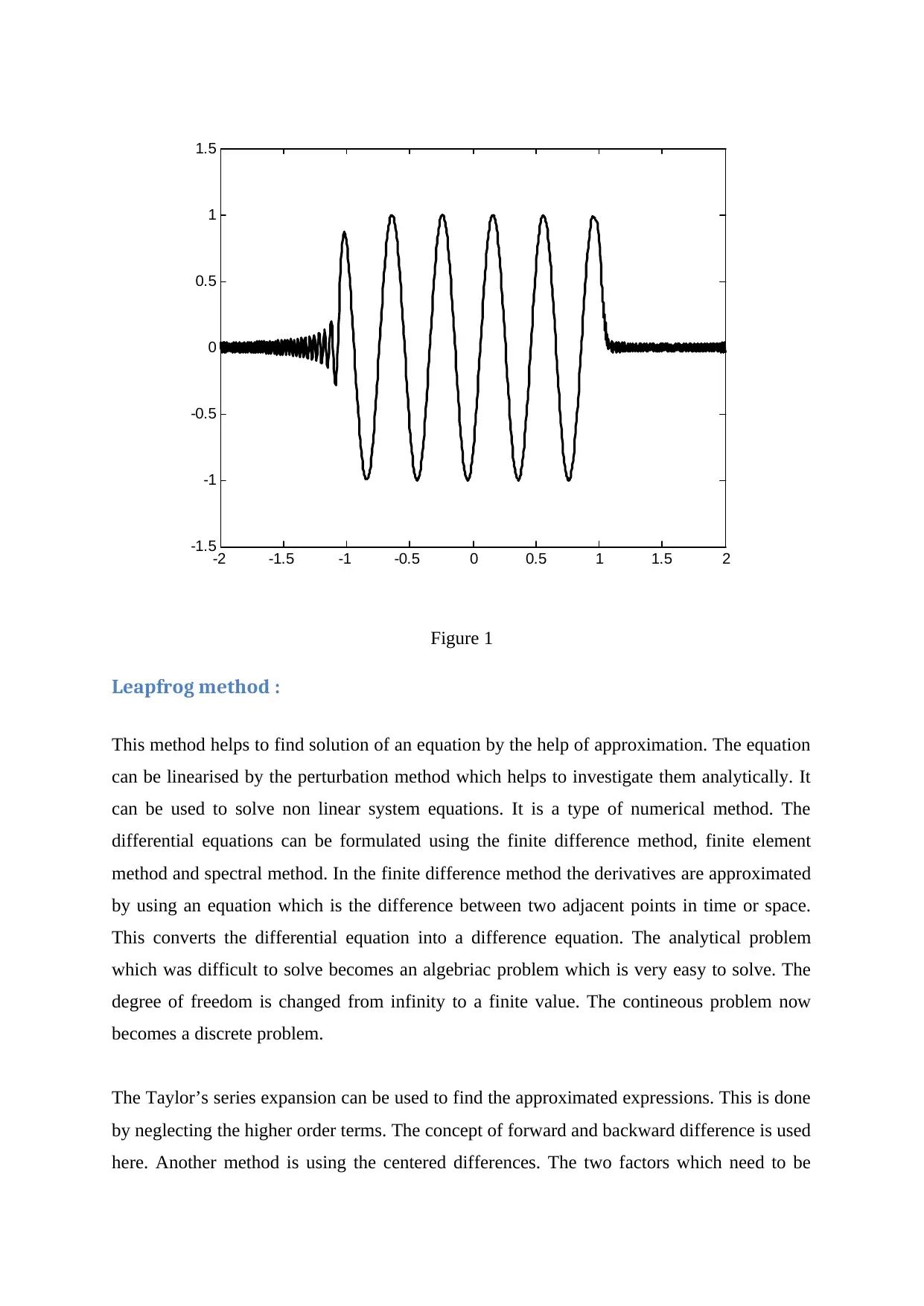
The solution to equation 1 is found and its evolution for t > 0 is investigated. The equation is
discretised to make it second-order accurate in time and space using the Leapfrog scheme.
U k+1, j – 2 Ukj + Uk-1j / ( ∆t ) 2 = Ukj-1 - 2Ukj + Ukj+1 ( ∆x ) 2 : (3)
At the computational end points, that is x = + / - 2, the boundary conditions considered are :
Minimal numerical reflections off the outer boundaries; i.e. the waves pass through the
boundaries and the solid wall condition.
By the help of proper calculations, the accuracy of the numerical solution is investigated,
discussed and demonstrated. The plot shows the basic features. The equation 3 represents the
modified PDE which gives an optimal value of the discretisation parameters giving the most
exact solution. The discrete dissipation-dispersion analysis helps to explain the numerical
observations.
Here, the solution of 1 – D wave equation is found by using the Leap frog scheme. The
boundary conditions provided have been used.
The one-dimensional wave equation for u ( x ; t ) is represented as follows :
utt = uxx ; ( 1 )
Here, x represents a spatial coordinate and t represents the time.
The initial conditions are given by :
At t = 0,
U ( x ; 0 ) = cos ( ∏ x / 2 δ )
. du / dt ( x ; 0 ) = 0; for -δ < = x < = δ ; ( 2 )
At other points when x > + / - δ and t = 0, u ( x , 0 ) = du / dt = 0.
Here, this equation is solved numerically for the domain x < = + / - 2, by taking δ = 0.01, 0.1
and 0.5 (an arbitrary parameter ) ( Celledoni, 2012 ).
The solution to equation 1 is found and its evolution for t > 0 is investigated. The equation is
discretised to make it second-order accurate in time and space using the Leapfrog scheme.
U k+1, j – 2 Ukj + Uk-1j / ( ∆t ) 2 = Ukj-1 - 2Ukj + Ukj+1 ( ∆x ) 2 : (3)
At the computational end points, that is x = + / - 2, the boundary conditions considered are :
Minimal numerical reflections off the outer boundaries; i.e. the waves pass through the
boundaries and the solid wall condition.
By the help of proper calculations, the accuracy of the numerical solution is investigated,
discussed and demonstrated. The plot shows the basic features. The equation 3 represents the
modified PDE which gives an optimal value of the discretisation parameters giving the most
exact solution. The discrete dissipation-dispersion analysis helps to explain the numerical
observations.
-2 -1.5 -1 -0.5 0 0.5 1 1.5 2
-1.5
-1
-0.5
0
0.5
1
1.5
Figure 1
Leapfrog method :
This method helps to find solution of an equation by the help of approximation. The equation
can be linearised by the perturbation method which helps to investigate them analytically. It
can be used to solve non linear system equations. It is a type of numerical method. The
differential equations can be formulated using the finite difference method, finite element
method and spectral method. In the finite difference method the derivatives are approximated
by using an equation which is the difference between two adjacent points in time or space.
This converts the differential equation into a difference equation. The analytical problem
which was difficult to solve becomes an algebriac problem which is very easy to solve. The
degree of freedom is changed from infinity to a finite value. The contineous problem now
becomes a discrete problem.
The Taylor’s series expansion can be used to find the approximated expressions. This is done
by neglecting the higher order terms. The concept of forward and backward difference is used
here. Another method is using the centered differences. The two factors which need to be
⊘ This is a preview!⊘
Do you want full access?
Subscribe today to unlock all pages.
Trusted by 1+ million students worldwide
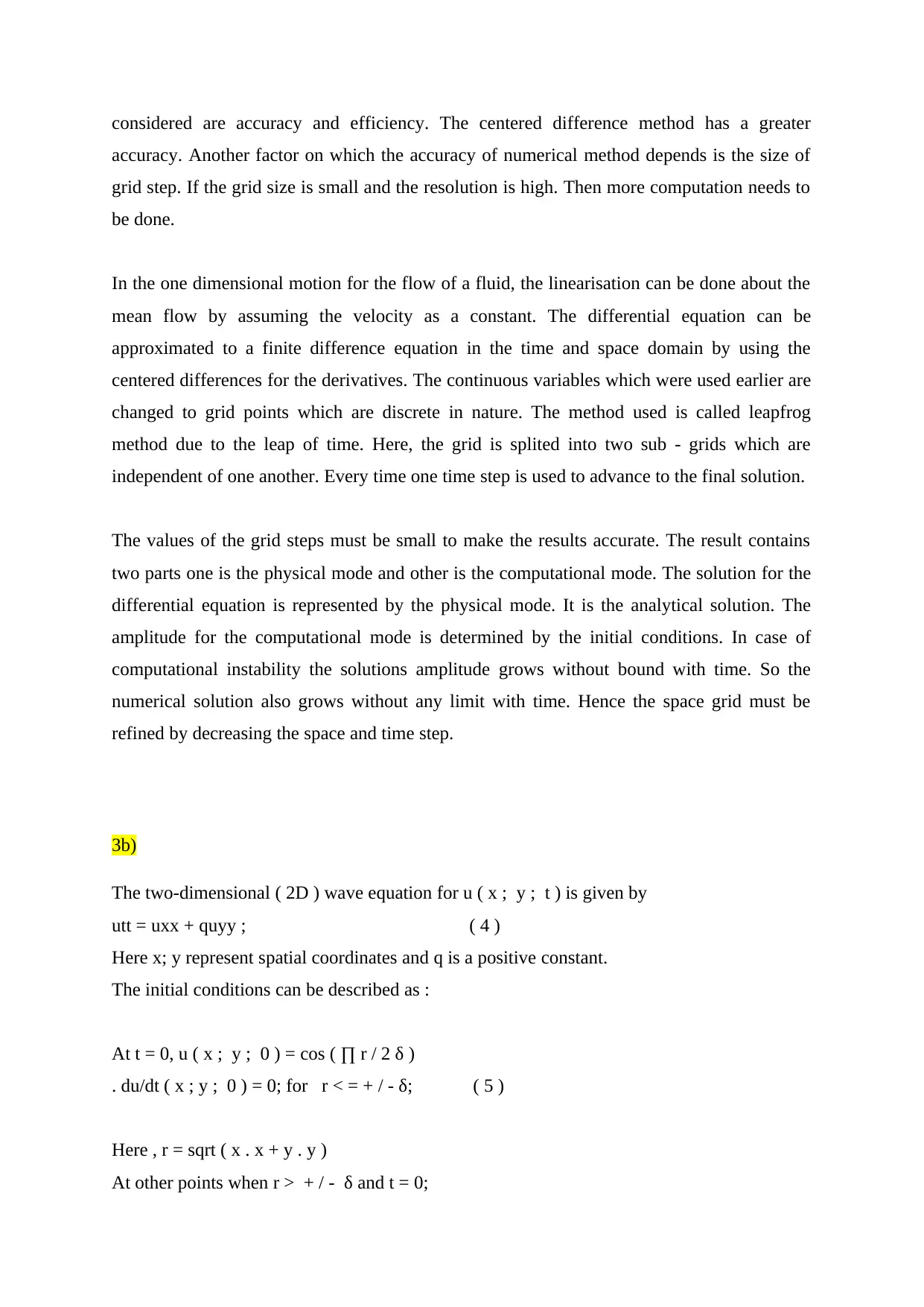
considered are accuracy and efficiency. The centered difference method has a greater
accuracy. Another factor on which the accuracy of numerical method depends is the size of
grid step. If the grid size is small and the resolution is high. Then more computation needs to
be done.
In the one dimensional motion for the flow of a fluid, the linearisation can be done about the
mean flow by assuming the velocity as a constant. The differential equation can be
approximated to a finite difference equation in the time and space domain by using the
centered differences for the derivatives. The continuous variables which were used earlier are
changed to grid points which are discrete in nature. The method used is called leapfrog
method due to the leap of time. Here, the grid is splited into two sub - grids which are
independent of one another. Every time one time step is used to advance to the final solution.
The values of the grid steps must be small to make the results accurate. The result contains
two parts one is the physical mode and other is the computational mode. The solution for the
differential equation is represented by the physical mode. It is the analytical solution. The
amplitude for the computational mode is determined by the initial conditions. In case of
computational instability the solutions amplitude grows without bound with time. So the
numerical solution also grows without any limit with time. Hence the space grid must be
refined by decreasing the space and time step.
3b)
The two-dimensional ( 2D ) wave equation for u ( x ; y ; t ) is given by
utt = uxx + quyy ; ( 4 )
Here x; y represent spatial coordinates and q is a positive constant.
The initial conditions can be described as :
At t = 0, u ( x ; y ; 0 ) = cos ( ∏ r / 2 δ )
. du/dt ( x ; y ; 0 ) = 0; for r < = + / - δ; ( 5 )
Here , r = sqrt ( x . x + y . y )
At other points when r > + / - δ and t = 0;
Paraphrase This Document
Need a fresh take? Get an instant paraphrase of this document with our AI Paraphraser
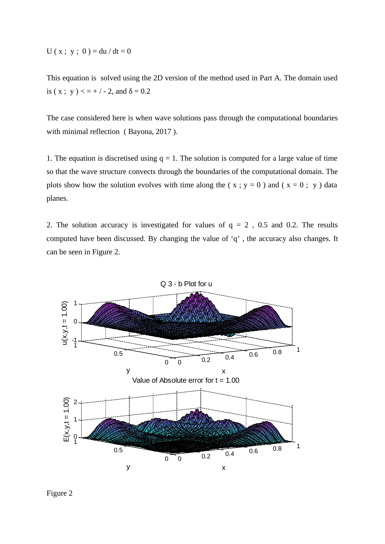
U ( x ; y ; 0 ) = du / dt = 0
This equation is solved using the 2D version of the method used in Part A. The domain used
is ( x ; y ) < = + / - 2, and δ = 0.2
The case considered here is when wave solutions pass through the computational boundaries
with minimal reflection ( Bayona, 2017 ).
1. The equation is discretised using q = 1. The solution is computed for a large value of time
so that the wave structure convects through the boundaries of the computational domain. The
plots show how the solution evolves with time along the ( x ; y = 0 ) and ( x = 0 ; y ) data
planes.
2. The solution accuracy is investigated for values of q = 2 , 0.5 and 0.2. The results
computed have been discussed. By changing the value of ‘q’ , the accuracy also changes. It
can be seen in Figure 2.
0 0.2 0.4 0.6 0.8 1
0
0.5
1
-1
0
1
x
Q 3 - b Plot for u
y
u(x,y,t = 1.00)
0 0.2 0.4 0.6 0.8 1
0
0.5
1
0
1
2
x
Value of Absolute error for t = 1.00
y
E(x,y,t = 1.00)
Figure 2
Second order equation
The leap frog method is used here which uses the centered second differences of time and
space. The accuracy and stability can be determined for the system. In order to use this
method for second order systems, a staggered mesh must be used. In this method the
significance of mesh increases due to an increase in the number of dimensions. The finite
volume method is used to solve them.
Initially, the variables are separated. The second order equation generates two solutions. The
initial conditions as well as the boundary conditions are used to determine the final solution.
The leapfrog method using the central differences is used to approximate the second order
partial derivatives. The time difference is made to leap over the space difference. The
movement is in the forward direction of time. The initial conditions must be satisfied by the
difference equation developed for the complete interval. This is necessary to make the
solution convergent. If a solution is convergent it must be stable also. The leapfrog method
can be applied to one way equation also. When a continuous system is converted into a
discrete system, the properties must not be lost.
The method used for centering of both the first order equation is the staggered grid method.
For a discretisation to be good the boundary conditions must be of absorbing type. If layer is
perfectly matched, then the coefficients can be chosen in such a manner that there is
minimum reflection at the boundary. A rectangular grid has the disadvantage that there is
more adaptability of the finite elements. But the FDTD method uses a large number of mesh
points. Hence a structured mesh has to be used. Numerical dispersion also occurs due to finite
differences. The value of the wave number decides the speed of the discrete wave. If the
errors caused due to dispersion are large. Then fourth order accuracy can be used for spatial
differences. This can be done by increasing the number of mesh values. This method will
increase the accuracy of the system but make it more complex. Another method is by
⊘ This is a preview!⊘
Do you want full access?
Subscribe today to unlock all pages.
Trusted by 1+ million students worldwide
increasing the time step. This has a drawback of making the system slow and also makes the
coding tough.
4.1)
Biconvex airfoil
To find the compressible flow characteristics around a biconvex airfoil for two dimensional
space numerical computation must be used. The equation used for this purpose is the Navier-
stoke’s equation ( Reynold averaged ).
The results obtained for a shock boundary layer depend on two factors. They are – mach
number and Reynolds number. The differential equations can be converted to discrete form in
space by the finite volume method. For second order scheme, the time can be advanced using
Euler backward method for second order. The boundary conditions are decided according to
the air foils. The important parameters of an airfoil are the cord length, thickness and the
radius of circular arc. The complete domain can be converted into a discrete mesh which
consists of several grids. This gives a solution which is independent of the grid.
The numerical computation helps to study the field characteristics of a compressible flow
around a biconvex airfoil. The flow field shows a steady state with small shock wave or
compression waves. A transient shock boundary layer interaction is also observed if the
pressure is low the fields flow becomes unstable.
The equation which describes a compressible fluid flowing over a surface is
given by :
d ( p ( 1 + u ) ) / dx + d ( p v ) / dy = 0 (6)
Here x; y represent spatial coordinates and ( u ; v ) are the velocity perturbations given by the
velocity potential ϕ;
. dϕ / dx = u and dϕ / dy = v (7)
The density p’ = 1 + p is given by
. p’ = 1 + p = ( 1 – y-1 / 2 . M2 ( 2 u + u2 + v2 ) ) 1 / y - 1 (8)
Paraphrase This Document
Need a fresh take? Get an instant paraphrase of this document with our AI Paraphraser
Hre, y = 1:4 and M is the Mach number.
‘p’ represents the density perturbation which tends to zero far away from the biconvex
surface and when M = 0, p = 0 throughout the computational field ( Pletcher, 2012 ).
.
The symmetrical biconvex aerofoil yb ( x ) is given by
Yb ( x ) = 2ґx ( 1 – x ); 0 <= x <= 1 (9)
Here, ґ denotes the maximum thickness of yb. The inviscid flow tangency condition on the
surface yb ( x ) is transferred to y = 0. Hence, for ґ << 1,
. dϕ / dy – ( 1 + dϕ / dx ) dyb / dx = 0 , 0 <=x <=1 for y = 0 (10)
On either side of the aerofoil, i.e. y = 0 a flow symmetry condition of
. dϕ / dy = dp / dy = 0; for x < 0 and x > 1; (11)
It is true if y tends to infinity and the normal velocity v tends to 0. If x tends to infinity
( positive or negative ), then the streamwise potential dϕ / dx tends to 0. For all the
boundaries, p is assumed to be tending to 0 ( Yang, 2018 ).
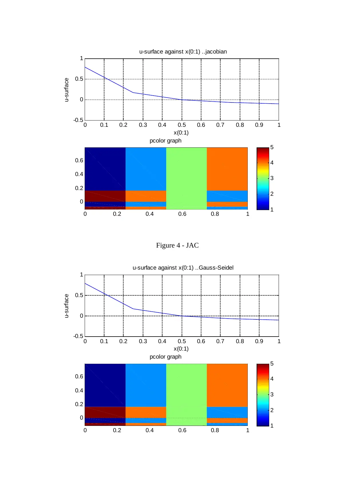
A numerical strategy has been devised to solve Eqn. (6). The method is based on guessing a
starting solution for p, which is then corrected during an iterative solution process. The
solutions are computed for ґ = 0:05. The Gauss-Seidel or SOR approach can be used.
4.2)
The numerical solutions are computed for M = 0.01, 0.2 and 0.4. The plots of the surface
velocity perturbation component are made.
Usurf = u = dϕ/dx on the aerofoil surface for 0 <= x <= 1 varies when M increases
( Benamou, 2014 ).
The plots are made to show the variation of Usurf varies with x(0 : 1) and along the entire y =
0; x(-q : s) plane. Also, the plots have been made of the surface v- velocity and density p
components along y = 0. A colour plot of the entire (u; v) and p perturbation field solutions
over your complete (x; y) computational domain have been made using the pcolor Matlab
command.
‘p’ represents the density perturbation which tends to zero far away from the biconvex
surface and when M = 0, p = 0 throughout the computational field ( Pletcher, 2012 ).
.
The symmetrical biconvex aerofoil yb ( x ) is given by
Yb ( x ) = 2ґx ( 1 – x ); 0 <= x <= 1 (9)
Here, ґ denotes the maximum thickness of yb. The inviscid flow tangency condition on the
surface yb ( x ) is transferred to y = 0. Hence, for ґ << 1,
. dϕ / dy – ( 1 + dϕ / dx ) dyb / dx = 0 , 0 <=x <=1 for y = 0 (10)
On either side of the aerofoil, i.e. y = 0 a flow symmetry condition of
. dϕ / dy = dp / dy = 0; for x < 0 and x > 1; (11)
It is true if y tends to infinity and the normal velocity v tends to 0. If x tends to infinity
( positive or negative ), then the streamwise potential dϕ / dx tends to 0. For all the
boundaries, p is assumed to be tending to 0 ( Yang, 2018 ).
A numerical strategy has been devised to solve Eqn. (6). The method is based on guessing a
starting solution for p, which is then corrected during an iterative solution process. The
solutions are computed for ґ = 0:05. The Gauss-Seidel or SOR approach can be used.
4.2)
The numerical solutions are computed for M = 0.01, 0.2 and 0.4. The plots of the surface
velocity perturbation component are made.
Usurf = u = dϕ/dx on the aerofoil surface for 0 <= x <= 1 varies when M increases
( Benamou, 2014 ).
The plots are made to show the variation of Usurf varies with x(0 : 1) and along the entire y =
0; x(-q : s) plane. Also, the plots have been made of the surface v- velocity and density p
components along y = 0. A colour plot of the entire (u; v) and p perturbation field solutions
over your complete (x; y) computational domain have been made using the pcolor Matlab
command.
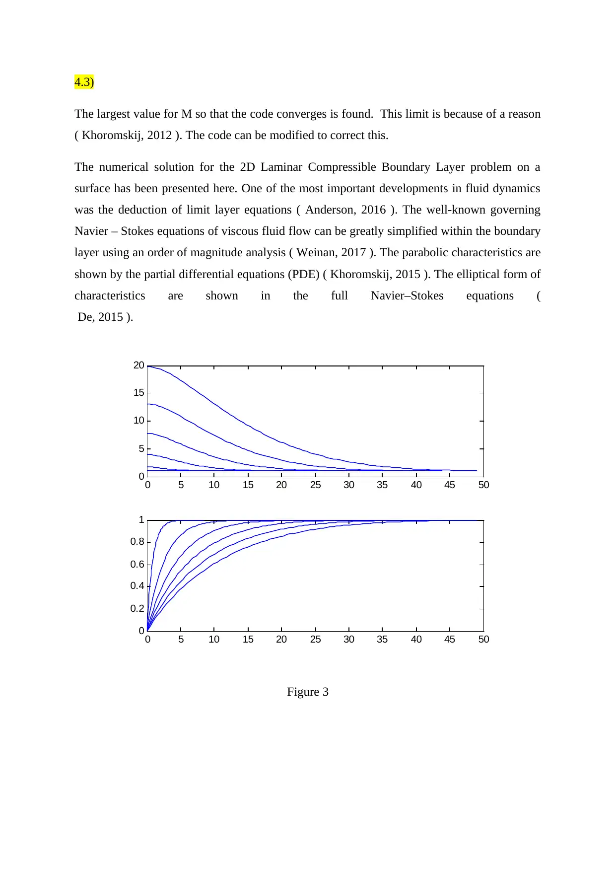
4.3)
The largest value for M so that the code converges is found. This limit is because of a reason
( Khoromskij, 2012 ). The code can be modified to correct this.
The numerical solution for the 2D Laminar Compressible Boundary Layer problem on a
surface has been presented here. One of the most important developments in fluid dynamics
was the deduction of limit layer equations ( Anderson, 2016 ). The well-known governing
Navier – Stokes equations of viscous fluid flow can be greatly simplified within the boundary
layer using an order of magnitude analysis ( Weinan, 2017 ). The parabolic characteristics are
shown by the partial differential equations (PDE) ( Khoromskij, 2015 ). The elliptical form of
characteristics are shown in the full Navier–Stokes equations (
De, 2015 ).
0 5 10 15 20 25 30 35 40 45 50
0
5
10
15
20
0 5 10 15 20 25 30 35 40 45 50
0
0.2
0.4
0.6
0.8
1
Figure 3
⊘ This is a preview!⊘
Do you want full access?
Subscribe today to unlock all pages.
Trusted by 1+ million students worldwide
0 0.1 0.2 0.3 0.4 0.5 0.6 0.7 0.8 0.9 1
-0.5
0
0.5
1
x(0:1)
u-surface
u-surface against x(0:1) ..jacobian
0 0.2 0.4 0.6 0.8 1
0
0.2
0.4
0.6
pcolor graph
1
2
3
4
5
Figure 4 - JAC
0 0.1 0.2 0.3 0.4 0.5 0.6 0.7 0.8 0.9 1
-0.5
0
0.5
1
x(0:1)
u-surface
u-surface against x(0:1) ..Gauss-Seidel
0 0.2 0.4 0.6 0.8 1
0
0.2
0.4
0.6
pcolor graph
1
2
3
4
5
-0.5
0
0.5
1
x(0:1)
u-surface
u-surface against x(0:1) ..jacobian
0 0.2 0.4 0.6 0.8 1
0
0.2
0.4
0.6
pcolor graph
1
2
3
4
5
Figure 4 - JAC
0 0.1 0.2 0.3 0.4 0.5 0.6 0.7 0.8 0.9 1
-0.5
0
0.5
1
x(0:1)
u-surface
u-surface against x(0:1) ..Gauss-Seidel
0 0.2 0.4 0.6 0.8 1
0
0.2
0.4
0.6
pcolor graph
1
2
3
4
5
Paraphrase This Document
Need a fresh take? Get an instant paraphrase of this document with our AI Paraphraser
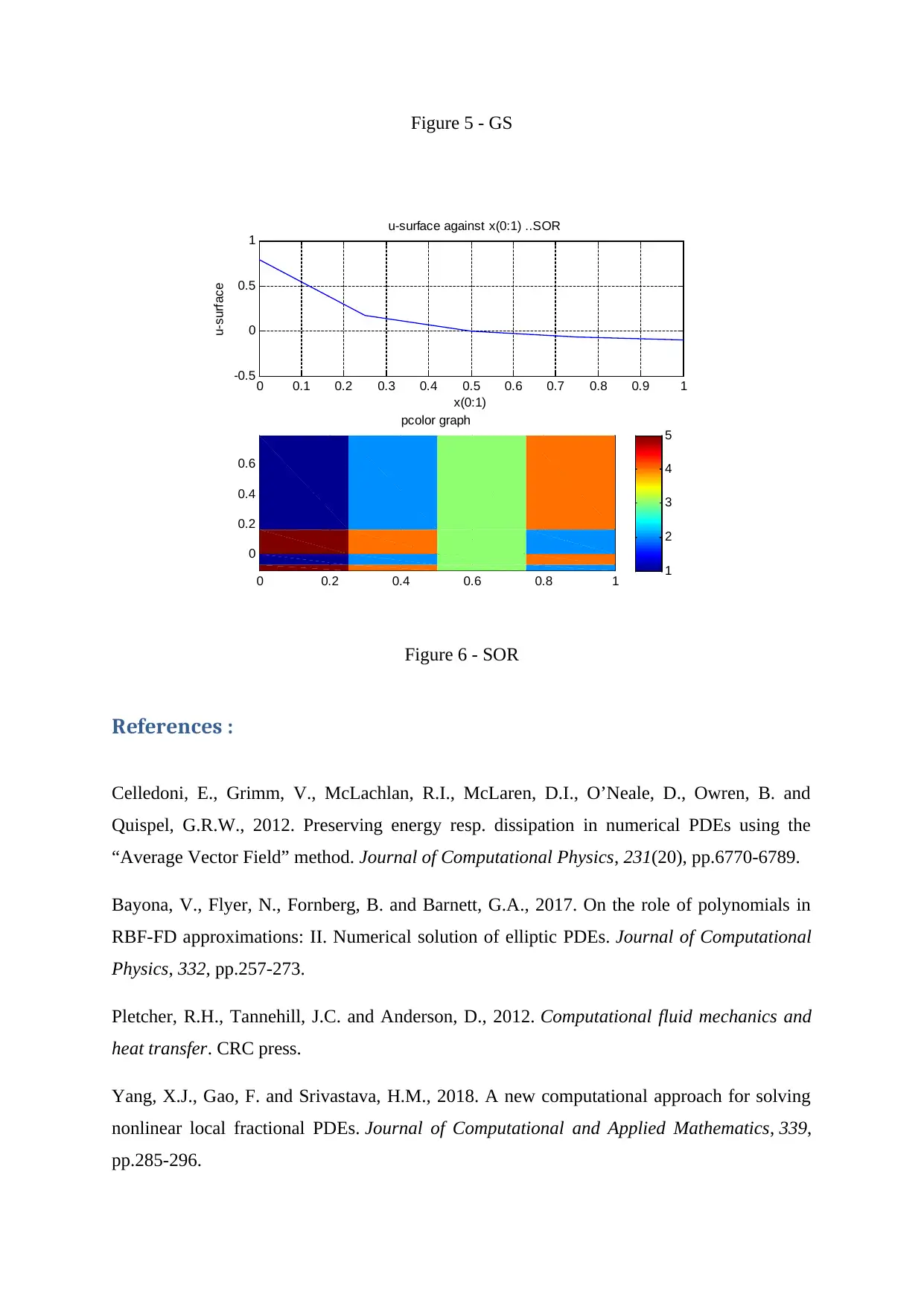
Figure 5 - GS
0 0.1 0.2 0.3 0.4 0.5 0.6 0.7 0.8 0.9 1
-0.5
0
0.5
1
x(0:1)
u-surface
u-surface against x(0:1) ..SOR
0 0.2 0.4 0.6 0.8 1
0
0.2
0.4
0.6
pcolor graph
1
2
3
4
5
Figure 6 - SOR
References :
Celledoni, E., Grimm, V., McLachlan, R.I., McLaren, D.I., O’Neale, D., Owren, B. and
Quispel, G.R.W., 2012. Preserving energy resp. dissipation in numerical PDEs using the
“Average Vector Field” method. Journal of Computational Physics, 231(20), pp.6770-6789.
Bayona, V., Flyer, N., Fornberg, B. and Barnett, G.A., 2017. On the role of polynomials in
RBF-FD approximations: II. Numerical solution of elliptic PDEs. Journal of Computational
Physics, 332, pp.257-273.
Pletcher, R.H., Tannehill, J.C. and Anderson, D., 2012. Computational fluid mechanics and
heat transfer. CRC press.
Yang, X.J., Gao, F. and Srivastava, H.M., 2018. A new computational approach for solving
nonlinear local fractional PDEs. Journal of Computational and Applied Mathematics, 339,
pp.285-296.
Anderson, D., Tannehill, J.C. and Pletcher, R.H., 2016. Computational fluid mechanics and
heat transfer. Taylor & Francis.
Weinan, E., Han, J. and Jentzen, A., 2017. Deep learning-based numerical methods for high-
dimensional parabolic partial differential equations and backward stochastic differential
equations. Communications in Mathematics and Statistics, 5(4), pp.349-380.
De los Reyes, J.C., 2015. Numerical PDE-constrained optimization. Springer.
Khoromskij, B.N., 2012. Tensors-structured numerical methods in scientific computing:
Survey on recent advances. Chemometrics and Intelligent Laboratory Systems, 110(1), pp.1-
19.
Benamou, J.D., Froese, B.D. and Oberman, A.M., 2014. Numerical solution of the optimal
transportation problem using the Monge–Ampère equation. Journal of Computational
Physics, 260, pp.107-126.
Khoromskij, B.N., 2015. Tensor numerical methods for multidimensional PDEs: theoretical
analysis and initial applications. ESAIM: Proceedings and Surveys, 48, pp.1-28.
⊘ This is a preview!⊘
Do you want full access?
Subscribe today to unlock all pages.
Trusted by 1+ million students worldwide
1 out of 12
Related Documents


Your All-in-One AI-Powered Toolkit for Academic Success.
+13062052269
info@desklib.com
Available 24*7 on WhatsApp / Email
![[object Object]](/_next/static/media/star-bottom.7253800d.svg)
Unlock your academic potential
Copyright © 2020–2026 A2Z Services. All Rights Reserved. Developed and managed by ZUCOL.