Optimizing Simultaneous Decisions | Assignment

1
Optimizing Simultaneous Decisions
Student Name
Institution Name
Date

2
Part A
Decision making scenario
Linear programming can be applied in a business set up to obtain the best way of
maximizing profits or minimizing the operational costs. In this case the decision-making
scenario involves production planning. To optimize production where various goods are to be
manufactured, the firm can apply linear programming to decide on the optimal quantity of each
product that ought to be produced taking into account the various constraints (Akpan & Iwok,
2016). The business scenario in question is making furniture (chairs, beds, tables). The decision
to be made is how many of each item should be produced by the firm in a given month to
maximize the profits.
Best initial gauze
In this business scenario the objective is to maximize the total profits from the furniture
production. The decision variables are the number of chairs, tables and beds that are to be
produced in a given month. Due to policy, resource and market limitation the decision will be
faced by a number of constraints some of them include:
Units produced should not be below the demanded units.
Production cost should be in line with the allocated capital.
Production hours should be less or equal to the available hours.
Tactical decision making
One tactical decision that will be dine after obtaining the optimal solution is sensitivity
analysis. This will be carried out to estimate how changes in the various aspects of production
will influence the total profit obtained.
Part B
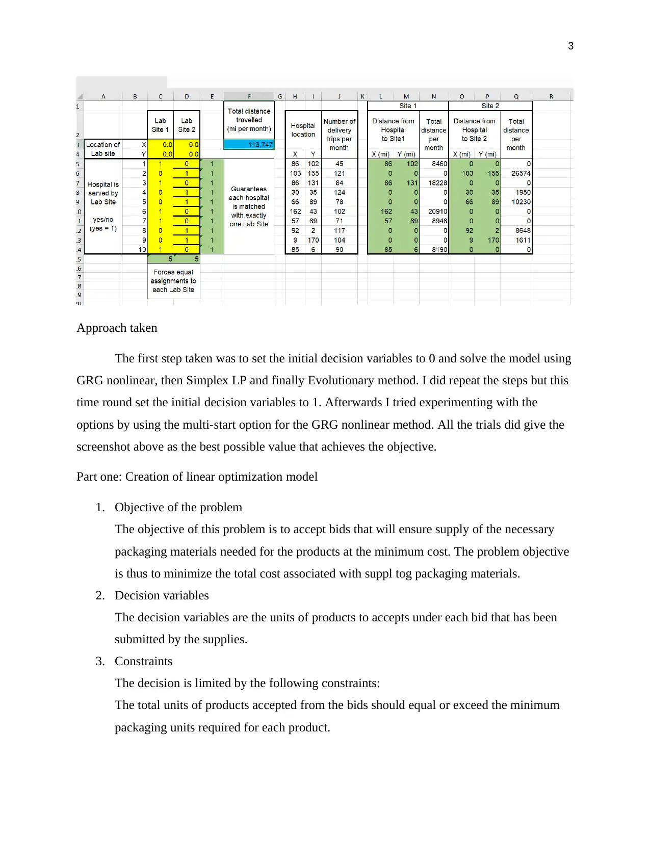
Screenshot of best result

3
Approach taken
The first step taken was to set the initial decision variables to 0 and solve the model using
GRG nonlinear, then Simplex LP and finally Evolutionary method. I did repeat the steps but this
time round set the initial decision variables to 1. Afterwards I tried experimenting with the
options by using the multi-start option for the GRG nonlinear method. All the trials did give the
screenshot above as the best possible value that achieves the objective.
Part one: Creation of linear optimization model
1. Objective of the problem
The objective of this problem is to accept bids that will ensure supply of the necessary
packaging materials needed for the products at the minimum cost. The problem objective
is thus to minimize the total cost associated with suppl tog packaging materials.
2. Decision variables
The decision variables are the units of products to accepts under each bid that has been
submitted by the supplies.
3. Constraints
The decision is limited by the following constraints:
The total units of products accepted from the bids should equal or exceed the minimum
packaging units required for each product.

4
Also, the quantity of packaging material to be accepted from a supplier should not exceed
the maximum units the supplier has committed to produce.
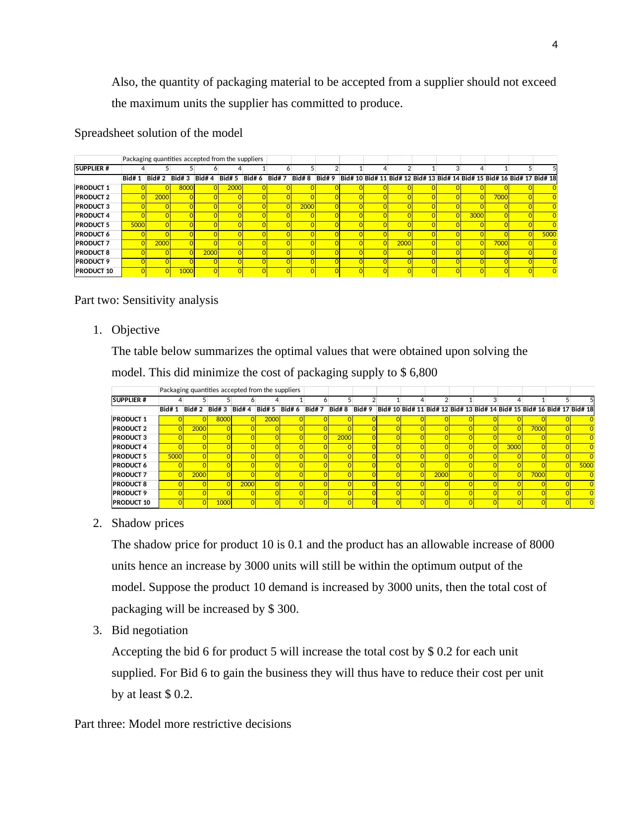
Spreadsheet solution of the model
Packaging quantities accepted from the suppliers
SUPPLIER # 4 5 5 6 4 1 6 5 2 1 4 2 1 3 4 1 5 5
Bid# 1 Bid# 2 Bid# 3 Bid# 4 Bid# 5 Bid# 6 Bid# 7 Bid# 8 Bid# 9 Bid# 10 Bid# 11 Bid# 12 Bid# 13 Bid# 14 Bid# 15 Bid# 16 Bid# 17 Bid# 18
PRODUCT 1 0 0 8000 0 2000 0 0 0 0 0 0 0 0 0 0 0 0 0
PRODUCT 2 0 2000 0 0 0 0 0 0 0 0 0 0 0 0 0 7000 0 0
PRODUCT 3 0 0 0 0 0 0 0 2000 0 0 0 0 0 0 0 0 0 0
PRODUCT 4 0 0 0 0 0 0 0 0 0 0 0 0 0 0 3000 0 0 0
PRODUCT 5 5000 0 0 0 0 0 0 0 0 0 0 0 0 0 0 0 0 0
PRODUCT 6 0 0 0 0 0 0 0 0 0 0 0 0 0 0 0 0 0 5000
PRODUCT 7 0 2000 0 0 0 0 0 0 0 0 0 2000 0 0 0 7000 0 0
PRODUCT 8 0 0 0 2000 0 0 0 0 0 0 0 0 0 0 0 0 0 0
PRODUCT 9 0 0 0 0 0 0 0 0 0 0 0 0 0 0 0 0 0 0
PRODUCT 10 0 0 1000 0 0 0 0 0 0 0 0 0 0 0 0 0 0 0
Part two: Sensitivity analysis
1. Objective
The table below summarizes the optimal values that were obtained upon solving the
model. This did minimize the cost of packaging supply to $ 6,800
Packaging quantities accepted from the suppliers
SUPPLIER # 4 5 5 6 4 1 6 5 2 1 4 2 1 3 4 1 5 5
Bid# 1 Bid# 2 Bid# 3 Bid# 4 Bid# 5 Bid# 6 Bid# 7 Bid# 8 Bid# 9 Bid# 10 Bid# 11 Bid# 12 Bid# 13 Bid# 14 Bid# 15 Bid# 16 Bid# 17 Bid# 18
PRODUCT 1 0 0 8000 0 2000 0 0 0 0 0 0 0 0 0 0 0 0 0
PRODUCT 2 0 2000 0 0 0 0 0 0 0 0 0 0 0 0 0 7000 0 0
PRODUCT 3 0 0 0 0 0 0 0 2000 0 0 0 0 0 0 0 0 0 0
PRODUCT 4 0 0 0 0 0 0 0 0 0 0 0 0 0 0 3000 0 0 0
PRODUCT 5 5000 0 0 0 0 0 0 0 0 0 0 0 0 0 0 0 0 0
PRODUCT 6 0 0 0 0 0 0 0 0 0 0 0 0 0 0 0 0 0 5000
PRODUCT 7 0 2000 0 0 0 0 0 0 0 0 0 2000 0 0 0 7000 0 0
PRODUCT 8 0 0 0 2000 0 0 0 0 0 0 0 0 0 0 0 0 0 0
PRODUCT 9 0 0 0 0 0 0 0 0 0 0 0 0 0 0 0 0 0 0
PRODUCT 10 0 0 1000 0 0 0 0 0 0 0 0 0 0 0 0 0 0 0
2. Shadow prices
The shadow price for product 10 is 0.1 and the product has an allowable increase of 8000
units hence an increase by 3000 units will still be within the optimum output of the
model. Suppose the product 10 demand is increased by 3000 units, then the total cost of
packaging will be increased by $ 300.
3. Bid negotiation
Accepting the bid 6 for product 5 will increase the total cost by $ 0.2 for each unit
supplied. For Bid 6 to gain the business they will thus have to reduce their cost per unit
by at least $ 0.2.
Part three: Model more restrictive decisions

5
Section A: All or nothing
Step 1
1. Objective of the problem
The objective is to minimize the total cost from the supply of the packaging materials.
2. Decision variables
The decision variable is to accept or reject a bid.
3. Constraints
The constraints include:
Total products supplied by the bids should exceed the minimum quantities required for
each product.
Step 4
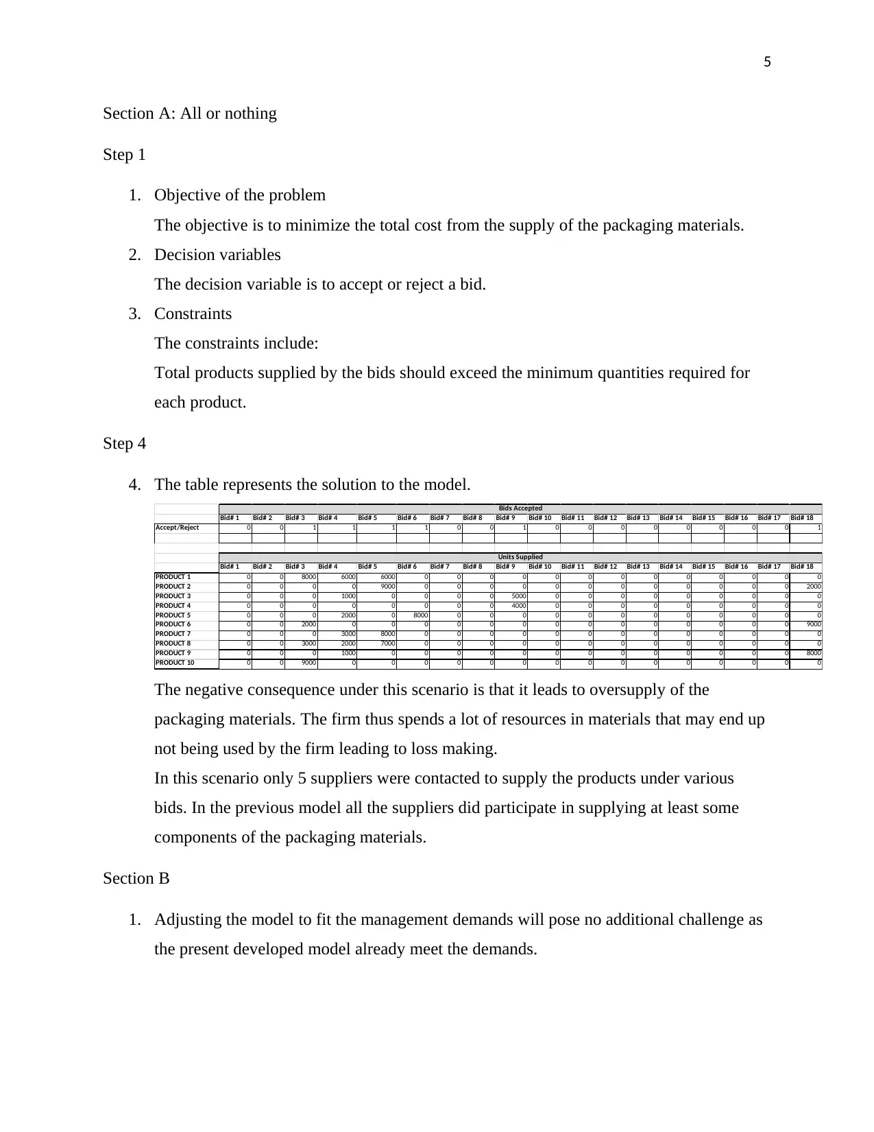
4. The table represents the solution to the model.
Bid# 1 Bid# 2 Bid# 3 Bid# 4 Bid# 5 Bid# 6 Bid# 7 Bid# 8 Bid# 9 Bid# 10 Bid# 11 Bid# 12 Bid# 13 Bid# 14 Bid# 15 Bid# 16 Bid# 17 Bid# 18
Accept/Reject 0 0 1 1 1 1 0 0 1 0 0 0 0 0 0 0 0 1
Bid# 1 Bid# 2 Bid# 3 Bid# 4 Bid# 5 Bid# 6 Bid# 7 Bid# 8 Bid# 9 Bid# 10 Bid# 11 Bid# 12 Bid# 13 Bid# 14 Bid# 15 Bid# 16 Bid# 17 Bid# 18
PRODUCT 1 0 0 8000 6000 6000 0 0 0 0 0 0 0 0 0 0 0 0 0
PRODUCT 2 0 0 0 0 9000 0 0 0 0 0 0 0 0 0 0 0 0 2000
PRODUCT 3 0 0 0 1000 0 0 0 0 5000 0 0 0 0 0 0 0 0 0
PRODUCT 4 0 0 0 0 0 0 0 0 4000 0 0 0 0 0 0 0 0 0
PRODUCT 5 0 0 0 2000 0 8000 0 0 0 0 0 0 0 0 0 0 0 0
PRODUCT 6 0 0 2000 0 0 0 0 0 0 0 0 0 0 0 0 0 0 9000
PRODUCT 7 0 0 0 3000 8000 0 0 0 0 0 0 0 0 0 0 0 0 0
PRODUCT 8 0 0 3000 2000 7000 0 0 0 0 0 0 0 0 0 0 0 0 0
PRODUCT 9 0 0 0 1000 0 0 0 0 0 0 0 0 0 0 0 0 0 8000
PRODUCT 10 0 0 9000 0 0 0 0 0 0 0 0 0 0 0 0 0 0 0
Bids Accepted
Units Supplied
The negative consequence under this scenario is that it leads to oversupply of the
packaging materials. The firm thus spends a lot of resources in materials that may end up
not being used by the firm leading to loss making.
In this scenario only 5 suppliers were contacted to supply the products under various
bids. In the previous model all the suppliers did participate in supplying at least some
components of the packaging materials.
Section B
1. Adjusting the model to fit the management demands will pose no additional challenge as
the present developed model already meet the demands.

6
References
Akpan, N. P. & Iwok, I., 2016. Application of Linear Programming for Optimal Use of Raw
Materials in Bakery. International Journal of Mathematics and Statistics Invention, 4(8), pp. 51-
57.