SOLUTION OF PARTIAL DIFFERENTIAL EQUATIONS BY FINITE DIFFERENCES

This document provides a solution to partial differential equations using the finite differences method. It includes MATLAB code and step-by-step instructions for solving the equations. The document also discusses the boundary conditions and initial conditions used in the calculations.

Running head: PARTIAL DIFFERENTIAL EQUATIONS
PARTIAL DIFFERENTIAL EQUATIONS
Name of the Student
Name of the University
Author Note

1SOLUTION OF PARTIAL DIFFERENTIAL EQUATIONS BY FINITE DIFFERENCES
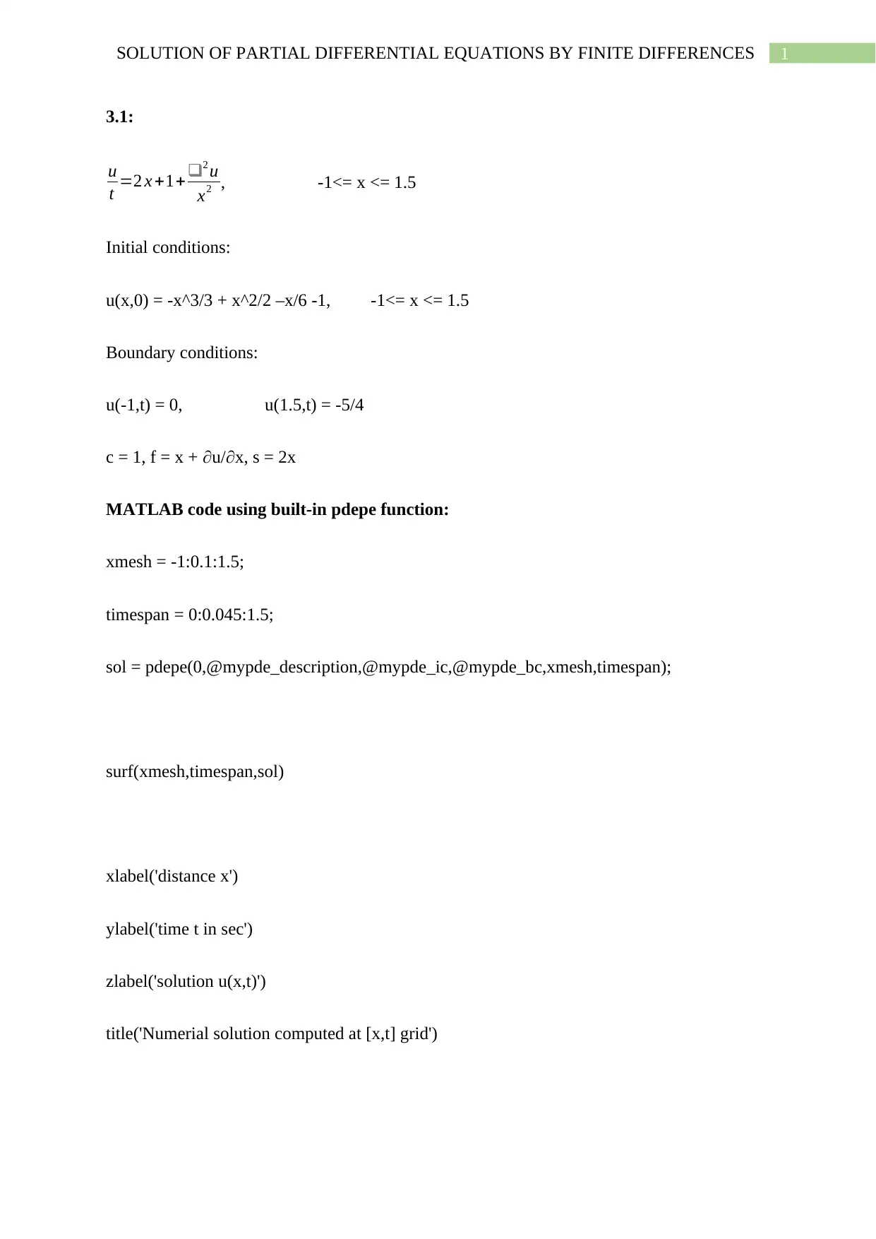
3.1:
u
t =2 x +1+❑2 u
x2 , -1<= x <= 1.5
Initial conditions:
u(x,0) = -x^3/3 + x^2/2 –x/6 -1, -1<= x <= 1.5
Boundary conditions:
u(-1,t) = 0, u(1.5,t) = -5/4
c = 1, f = x + u/x, s = 2x
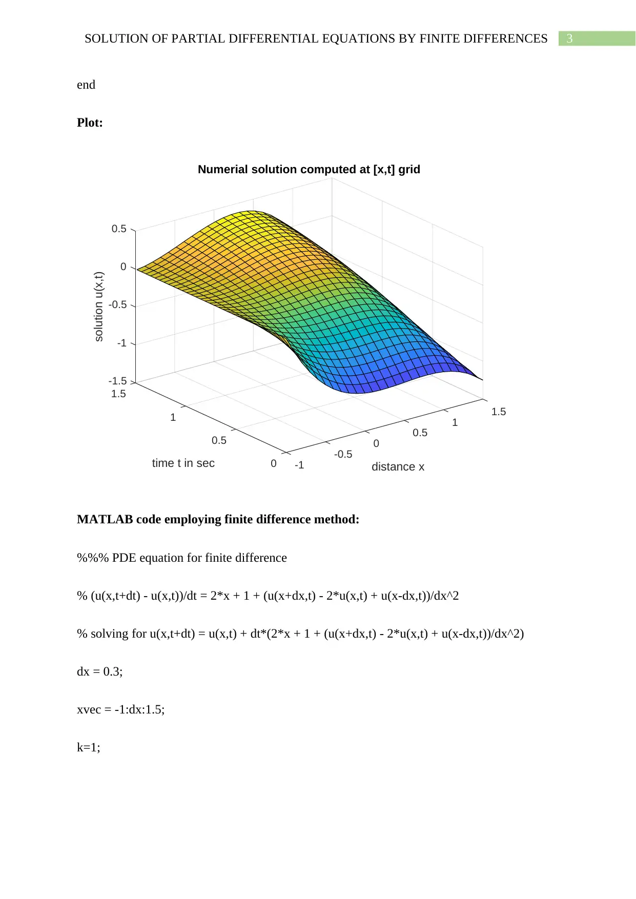
MATLAB code using built-in pdepe function:
xmesh = -1:0.1:1.5;
timespan = 0:0.045:1.5;
sol = pdepe(0,@mypde_description,@mypde_ic,@mypde_bc,xmesh,timespan);
surf(xmesh,timespan,sol)
xlabel('distance x')
ylabel('time t in sec')
zlabel('solution u(x,t)')
title('Numerial solution computed at [x,t] grid')

2SOLUTION OF PARTIAL DIFFERENTIAL EQUATIONS BY FINITE DIFFERENCES
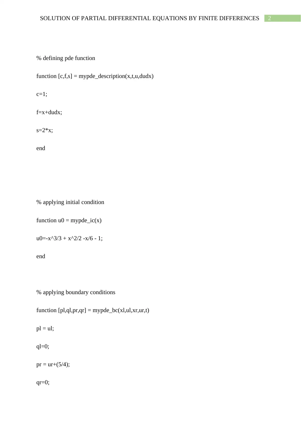
% defining pde function
function [c,f,s] = mypde_description(x,t,u,dudx)
c=1;
f=x+dudx;
s=2*x;
end
% applying initial condition
function u0 = mypde_ic(x)
u0=-x^3/3 + x^2/2 -x/6 - 1;
end
% applying boundary conditions
function [pl,ql,pr,qr] = mypde_bc(xl,ul,xr,ur,t)
pl = ul;
ql=0;
pr = ur+(5/4);
qr=0;

3SOLUTION OF PARTIAL DIFFERENTIAL EQUATIONS BY FINITE DIFFERENCES
end
Plot:
-1.5
1.5
-1
1.5
-0.5
solution u(x,t)
1 1
Numerial solution computed at [x,t] grid
0
time t in sec
0.5
distance x
0.5
0.5 0
-0.5
0 -1
MATLAB code employing finite difference method:
%%% PDE equation for finite difference
% (u(x,t+dt) - u(x,t))/dt = 2*x + 1 + (u(x+dx,t) - 2*u(x,t) + u(x-dx,t))/dx^2
% solving for u(x,t+dt) = u(x,t) + dt*(2*x + 1 + (u(x+dx,t) - 2*u(x,t) + u(x-dx,t))/dx^2)
dx = 0.3;
xvec = -1:dx:1.5;
k=1;

4SOLUTION OF PARTIAL DIFFERENTIAL EQUATIONS BY FINITE DIFFERENCES
dt = (dx^2)/(2*k); % employing stability criterion. dt <= dx^2/2k, where k is any positive
integer. k ~= 0.
tvec = 0:dt:1.5;
umat = zeros(length(xvec),length(tvec)); % initializing u(x,t) with zeros
% initial condition u(x,0) = -x^3/3 + x^2/2 - x/6 - 1 when -1<=x<=1.5
umat(:,1) = -(xvec.^3)./3 + (xvec.^2)./2 - xvec./6 - 1;
% Boundary Conditions
umat(1,:) = 0; % u(-1,t) = 0
umat(end,:) = -5/4; % u(1.5,t) = -5/4
% Employing finite difference formula
for tcount=1:length(tvec)-1
for xcount = 2:length(xvec) - 1
umat(xcount,tcount + 1) = umat(xcount,tcount) + k*dt*(2*xcount + 1 +
(umat(xcount+1,tcount) - 2*umat(xcount,tcount) + umat(xcount-1,tcount))/dx^2);
end

5SOLUTION OF PARTIAL DIFFERENTIAL EQUATIONS BY FINITE DIFFERENCES
end
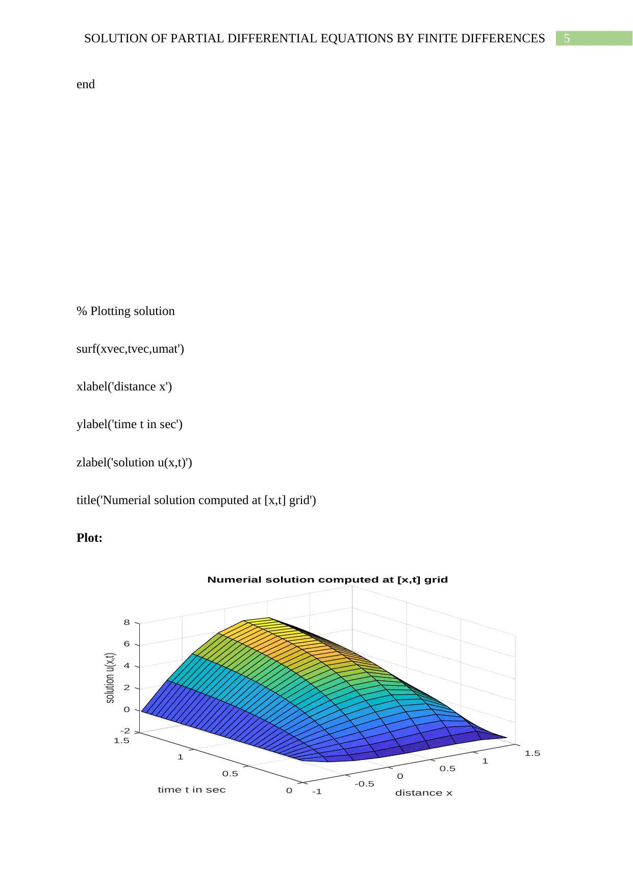
% Plotting solution
surf(xvec,tvec,umat')
xlabel('distance x')
ylabel('time t in sec')
zlabel('solution u(x,t)')
title('Numerial solution computed at [x,t] grid')
Plot:
-2
1.5
0
2
1.5
solution u(x,t)
1
4
1
Numerial solution computed at [x,t] grid
time t in sec
6
0.5
distance x
8
0.5 0
-0.5
0 -1

6SOLUTION OF PARTIAL DIFFERENTIAL EQUATIONS BY FINITE DIFFERENCES
Hence, the finite difference method approximately solves the partial differential equation,
however the u values are slightly larger than the values of obtained by employing pdepe
method.
Problem 3.2:
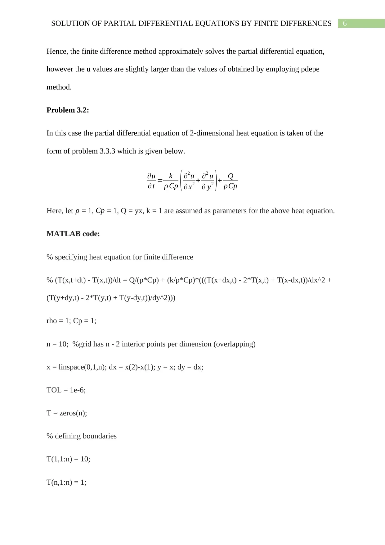
In this case the partial differential equation of 2-dimensional heat equation is taken of the
form of problem 3.3.3 which is given below.
∂u
∂ t = k
ρ Cp ( ∂2 u
∂ x2 + ∂2 u
∂ y2 ) + Q
ρCp
Here, let ρ = 1, Cp = 1, Q = yx, k = 1 are assumed as parameters for the above heat equation.
MATLAB code:
% specifying heat equation for finite difference
% (T(x,t+dt) - T(x,t))/dt = Q/(p*Cp) + (k/p*Cp)*(((T(x+dx,t) - 2*T(x,t) + T(x-dx,t))/dx^2 +
(T(y+dy,t) - 2*T(y,t) + T(y-dy,t))/dy^2)))
rho = 1; Cp = 1;
n = 10; %grid has n - 2 interior points per dimension (overlapping)
x = linspace(0,1,n); dx = x(2)-x(1); y = x; dy = dx;
TOL = 1e-6;
T = zeros(n);
% defining boundaries
T(1,1:n) = 10;
T(n,1:n) = 1;

7SOLUTION OF PARTIAL DIFFERENTIAL EQUATIONS BY FINITE DIFFERENCES
T(1:n,1) = 1;
T(1:n,n) = 1;
dt = dx^2/4;
error = 1; k = 0;
while error > TOL
k = k+1;
Told = T;
for i = 2:n-1
for j = 2:n-1
T(i,j) = (1/(rho*Cp))*dt*((Told(i+1,j)-2*Told(i,j)+Told(i-1,j))/dx^2 ...
+ (Told(i,j+1)-2*Told(i,j)+Told(i,j-1))/dy^2 + (i*j)/(rho*Cp)) ...
+ Told(i,j);
end
end
error = max(max(abs(Told-T)));
end
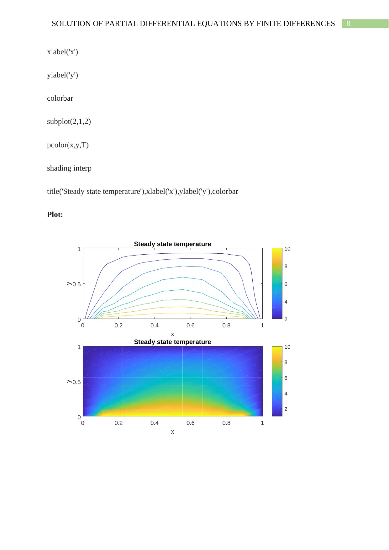
subplot(2,1,1),contour(x,y,T),
title('Steady state temperature')

8SOLUTION OF PARTIAL DIFFERENTIAL EQUATIONS BY FINITE DIFFERENCES
xlabel('x')
ylabel('y')
colorbar
subplot(2,1,2)
pcolor(x,y,T)
shading interp
title('Steady state temperature'),xlabel('x'),ylabel('y'),colorbar
Plot:
Steady state temperature
0 0.2 0.4 0.6 0.8 1
x
0
0.5
1
y
2
4
6
8
10
0 0.2 0.4 0.6 0.8 1
x
0
0.5
1
y
Steady state temperature
2
4
6
8
10

9SOLUTION OF PARTIAL DIFFERENTIAL EQUATIONS BY FINITE DIFFERENCES