Predict Business Results Question Answer 2022

Running head: STATISTICS 1
Predict Business Results
Student Name
Professor’s Name
University Name
Date

STATISTICS 2
Predict Business Results
Assessment Answers by (Insert your name here)
In the summary tables below, insert only the answers. You will show work after the summary
section.
Question 1 answers
1a: forecast $4812.7143
1b: reliability The value of significance F (0.037) is less than the default significance
level of 0.05. Hence, we are 95% confident that forecast made using the
regression model is accurate.
Question 2 answers
2a: formula Y =1.3232 β0 +0.0773 β1 −0.1700 β2 −1.5224 β3 +98.3291
Where Y is Job satisfaction, β0 is Relationship with supervisor, β1 is
opportunities for advancement, β2 is overall quality of work
environment, and β3 is total hours worked per week. The intercept is
98.3291.
2b: reliability The coefficient of determination is 0.823 (82.3% variation) and the
value of significance f is 3.74 x 10−5 and is less than 0.05 significance
level. Therefore, there is a 95% reliability that 82.3% of the estimate
will be based on the multiple regression formula.
2c: variables  Opportunities for Advancement
 Overall quality of work environment
They are not good predictors because they are not statistically

STATISTICS 3
significant.
2d: expected
score
Job satisfaction score is equal 49.4821 which can be rounded off to a
job satisfaction of 50.
Question 3 answers
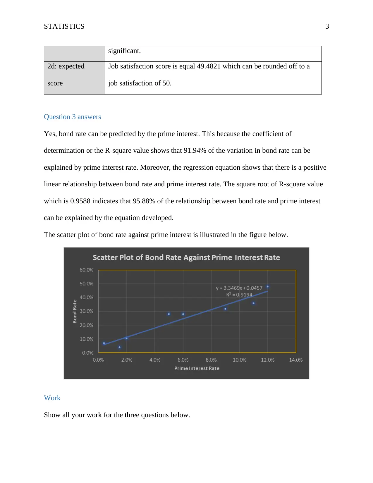
Yes, bond rate can be predicted by the prime interest. This because the coefficient of
determination or the R-square value shows that 91.94% of the variation in bond rate can be
explained by prime interest rate. Moreover, the regression equation shows that there is a positive
linear relationship between bond rate and prime interest rate. The square root of R-square value
which is 0.9588 indicates that 95.88% of the relationship between bond rate and prime interest
can be explained by the equation developed.
The scatter plot of bond rate against prime interest is illustrated in the figure below.
Work
Show all your work for the three questions below.

STATISTICS 4
Question 1
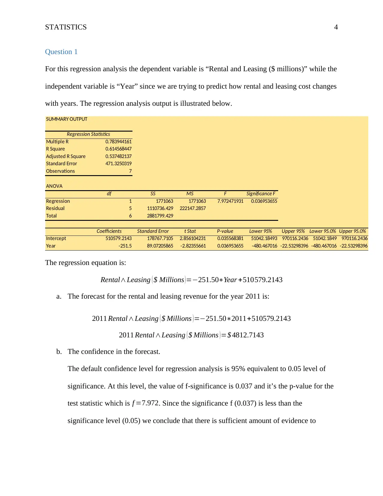
For this regression analysis the dependent variable is “Rental and Leasing ($ millions)” while the
independent variable is “Year” since we are trying to predict how rental and leasing cost changes
with years. The regression analysis output is illustrated below.
SUMMARY OUTPUT
Regression Statistics
Multiple R 0.783944161
R Square 0.614568447
Adjusted R Square 0.537482137
Standard Error 471.3250319
Observations 7
ANOVA
df SS MS F Significance F
Regression 1 1771063 1771063 7.972471931 0.036953655
Residual 5 1110736.429 222147.2857
Total 6 2881799.429
Coefficients Standard Error t Stat P-value Lower 95% Upper 95% Lower 95.0% Upper 95.0%
Intercept 510579.2143 178767.7105 2.856104231 0.035568381 51042.18493 970116.2436 51042.1849 970116.2436
Year -251.5 89.07205865 -2.82355661 0.036953655 -480.467016 -22.53298396 -480.467016 -22.53298396
The regression equation is:
Rental∧Leasing ( $ Millions )=−251.50∗Year +510579.2143
a. The forecast for the rental and leasing revenue for the year 2011 is:
2011 Rental∧Leasing ( $ Millions ) =−251.50∗2011+510579.2143
2011 Rental∧Leasing ( $ Millions )=$ 4812.7143
b. The confidence in the forecast.
The default confidence level for regression analysis is 95% equivalent to 0.05 level of
significance. At this level, the value of f-significance is 0.037 and it’s the p-value for the
test statistic which is f =7.972. Since the significance f (0.037) is less than the
significance level (0.05) we conclude that there is sufficient amount of evidence to

STATISTICS 5
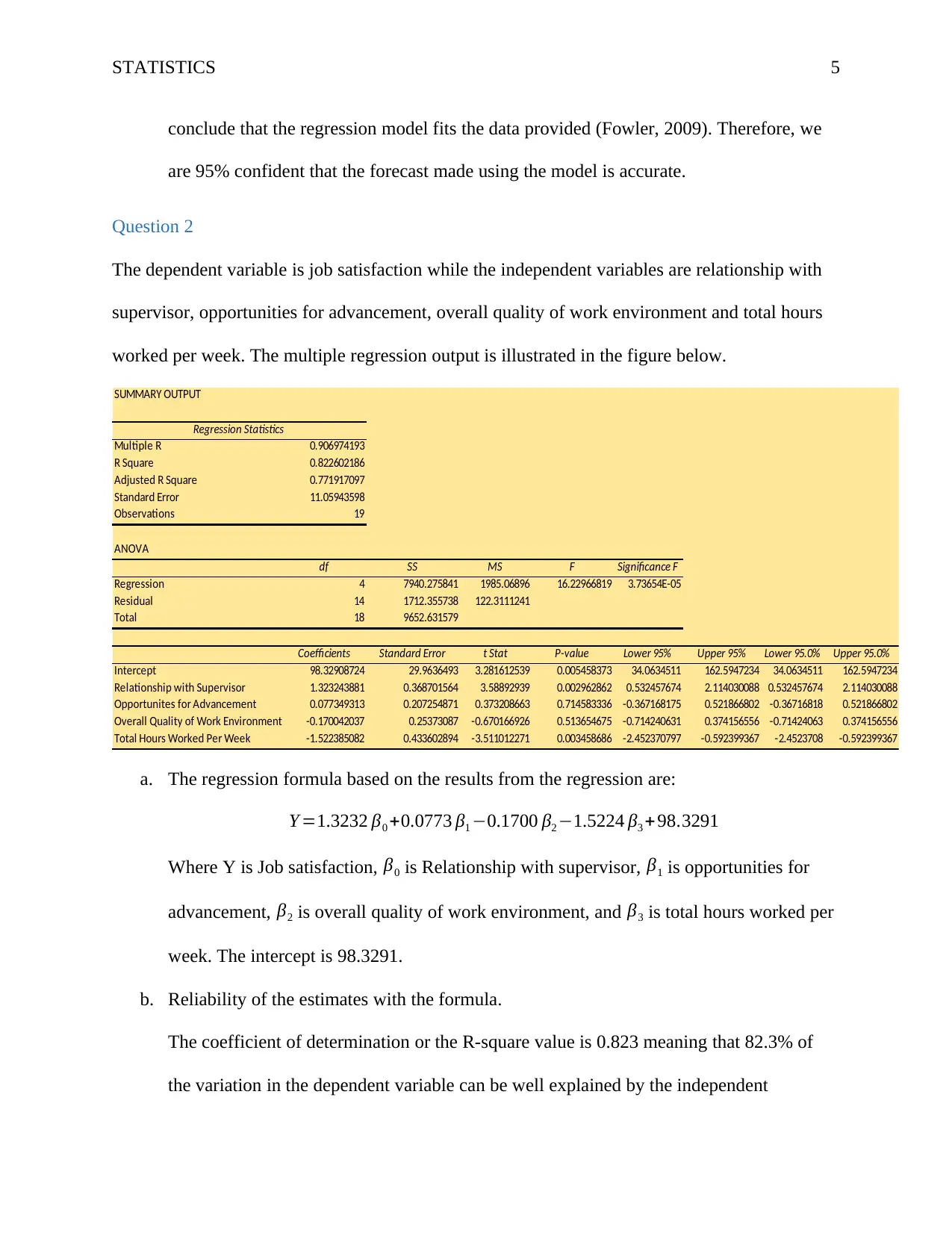
conclude that the regression model fits the data provided (Fowler, 2009). Therefore, we
are 95% confident that the forecast made using the model is accurate.
Question 2
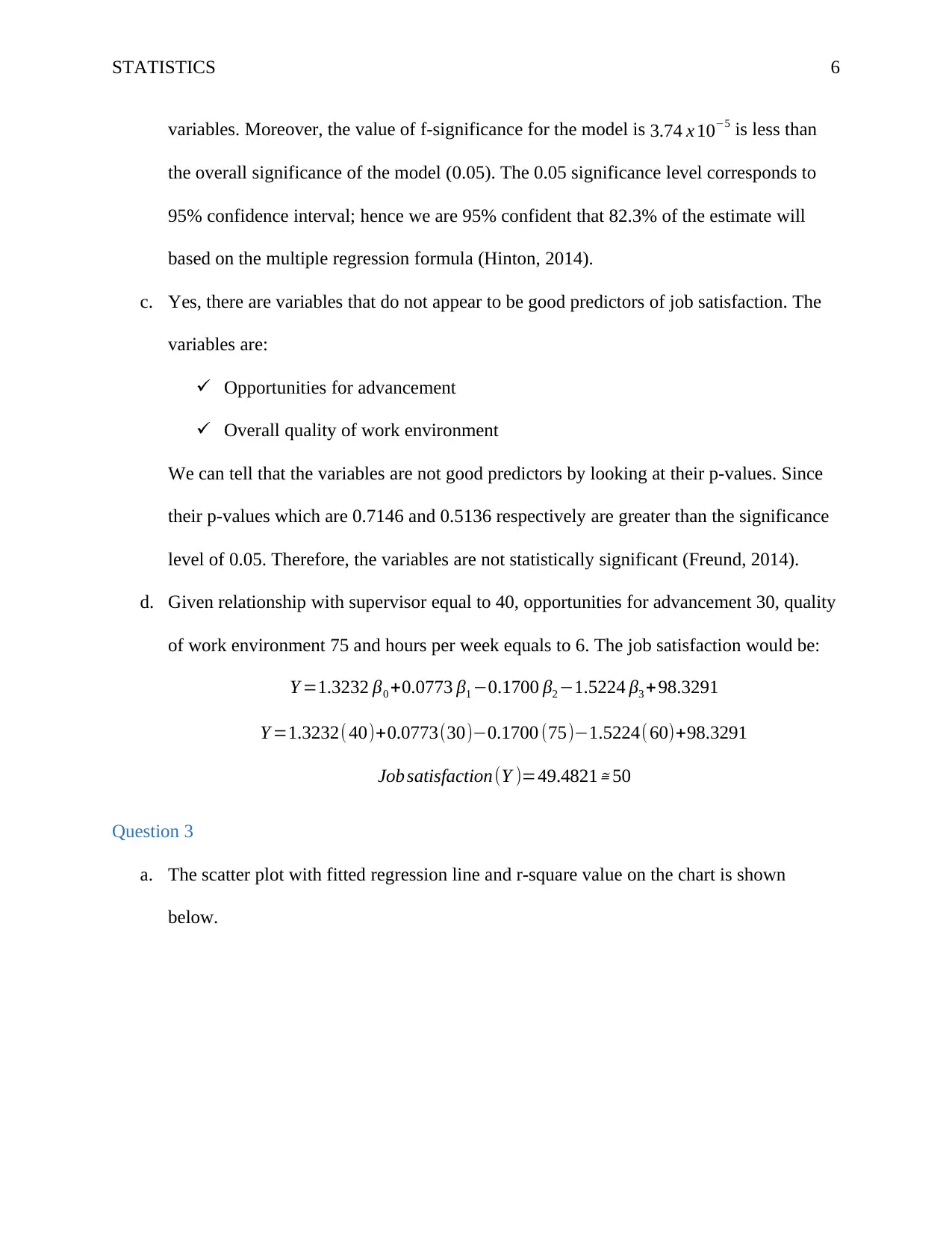
The dependent variable is job satisfaction while the independent variables are relationship with
supervisor, opportunities for advancement, overall quality of work environment and total hours
worked per week. The multiple regression output is illustrated in the figure below.
SUMMARY OUTPUT
Regression Statistics
Multiple R 0.906974193
R Square 0.822602186
Adjusted R Square 0.771917097
Standard Error 11.05943598
Observations 19
ANOVA
df SS MS F Significance F
Regression 4 7940.275841 1985.06896 16.22966819 3.73654E-05
Residual 14 1712.355738 122.3111241
Total 18 9652.631579
Coefficients Standard Error t Stat P-value Lower 95% Upper 95% Lower 95.0% Upper 95.0%
Intercept 98.32908724 29.9636493 3.281612539 0.005458373 34.0634511 162.5947234 34.0634511 162.5947234
Relationship with Supervisor 1.323243881 0.368701564 3.58892939 0.002962862 0.532457674 2.114030088 0.532457674 2.114030088
Opportunites for Advancement 0.077349313 0.207254871 0.373208663 0.714583336 -0.367168175 0.521866802 -0.36716818 0.521866802
Overall Quality of Work Environment -0.170042037 0.25373087 -0.670166926 0.513654675 -0.714240631 0.374156556 -0.71424063 0.374156556
Total Hours Worked Per Week -1.522385082 0.433602894 -3.511012271 0.003458686 -2.452370797 -0.592399367 -2.4523708 -0.592399367
a. The regression formula based on the results from the regression are:
Y =1.3232 β0 +0.0773 β1 −0.1700 β2 −1.5224 β3 + 98.3291
Where Y is Job satisfaction, β0 is Relationship with supervisor, β1 is opportunities for
advancement, β2 is overall quality of work environment, and β3 is total hours worked per
week. The intercept is 98.3291.
b. Reliability of the estimates with the formula.
The coefficient of determination or the R-square value is 0.823 meaning that 82.3% of
the variation in the dependent variable can be well explained by the independent

STATISTICS 6
variables. Moreover, the value of f-significance for the model is 3.74 x 10−5 is less than
the overall significance of the model (0.05). The 0.05 significance level corresponds to
95% confidence interval; hence we are 95% confident that 82.3% of the estimate will
based on the multiple regression formula (Hinton, 2014).
c. Yes, there are variables that do not appear to be good predictors of job satisfaction. The
variables are:
 Opportunities for advancement
 Overall quality of work environment
We can tell that the variables are not good predictors by looking at their p-values. Since
their p-values which are 0.7146 and 0.5136 respectively are greater than the significance
level of 0.05. Therefore, the variables are not statistically significant (Freund, 2014).
d. Given relationship with supervisor equal to 40, opportunities for advancement 30, quality
of work environment 75 and hours per week equals to 6. The job satisfaction would be:
Y =1.3232 β0 +0.0773 β1 −0.1700 β2 −1.5224 β3 +98.3291
Y =1.3232( 40)+0.0773(30)−0.1700 (75)−1.5224( 60)+98.3291
Job satisfaction(Y )=49.4821≅ 50
Question 3
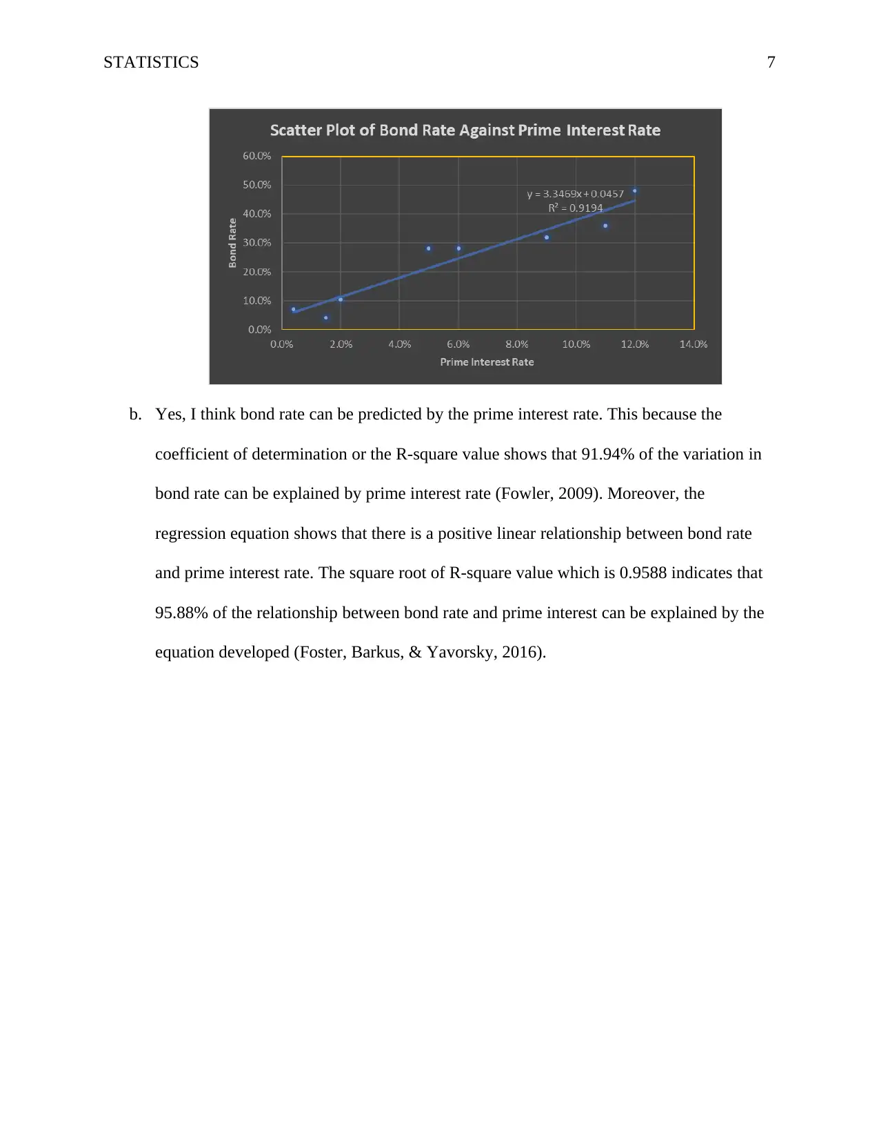
a. The scatter plot with fitted regression line and r-square value on the chart is shown
below.

STATISTICS 7
b. Yes, I think bond rate can be predicted by the prime interest rate. This because the
coefficient of determination or the R-square value shows that 91.94% of the variation in
bond rate can be explained by prime interest rate (Fowler, 2009). Moreover, the
regression equation shows that there is a positive linear relationship between bond rate
and prime interest rate. The square root of R-square value which is 0.9588 indicates that
95.88% of the relationship between bond rate and prime interest can be explained by the
equation developed (Foster, Barkus, & Yavorsky, 2016).

STATISTICS 8
References
Foster, J. J., Barkus, E., & Yavorsky, C., (2016). Understanding and using advanced statistics
(2nd ed). London: SAGE.
Fowler, F., (2009). Survey research methods. Thousand Oaks, Calif.: Sage.
Freund, J. E., (2014). Modern elementary statistics (12th ed). Boston: Pearson.
Hinton, P. R., (2014). Statistics explained (3rd ed). London: Routledge, Taylor & Francis Group.