The Propagation Constant Solution 2022
VerifiedAdded on 2022/09/18
|22
|556
|29
AI Summary
Contribute Materials
Your contribution can guide someone’s learning journey. Share your
documents today.
Part 1
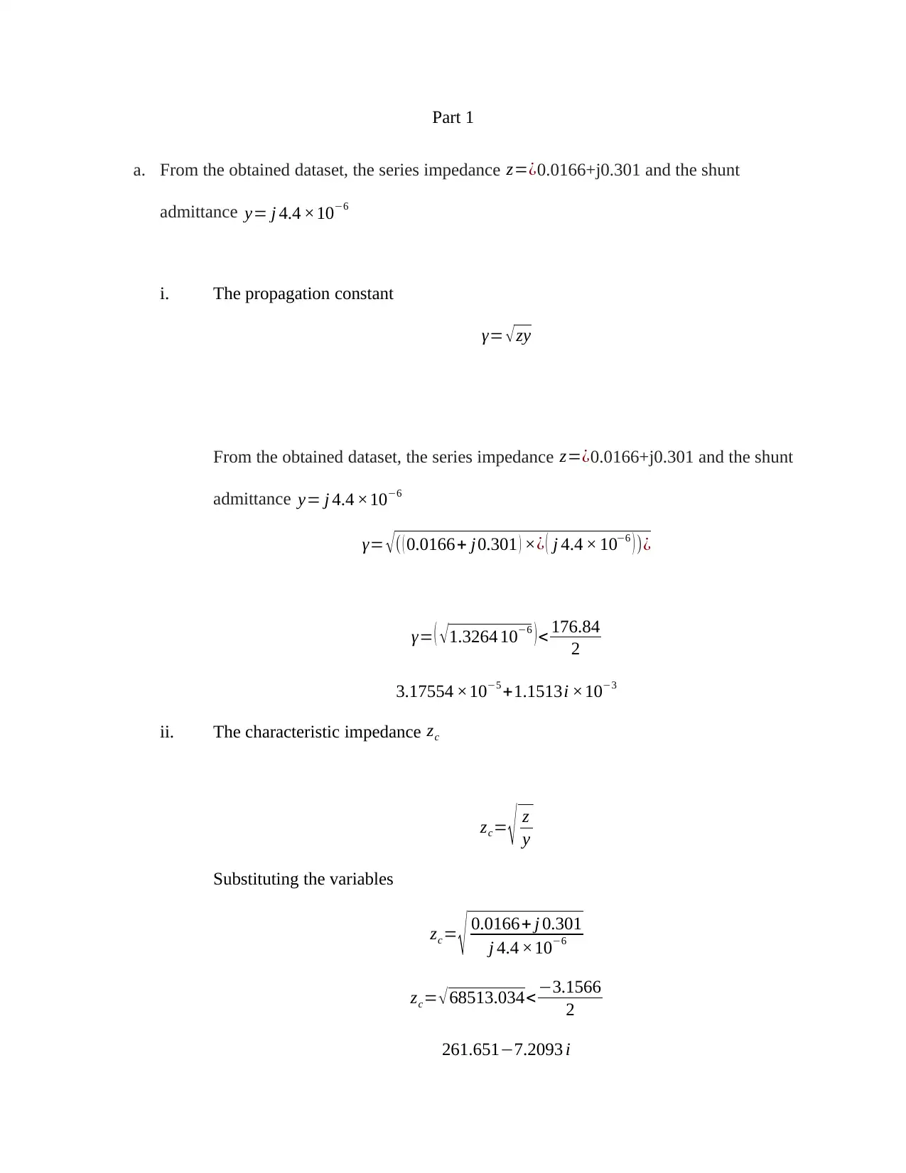
a. From the obtained dataset, the series impedance z=¿0.0166+j0.301 and the shunt
admittance y= j 4.4 ×10⁻⁶
i. The propagation constant
γ= √zy
From the obtained dataset, the series impedance z=¿0.0166+j0.301 and the shunt
admittance y= j 4.4 ×10⁻⁶
γ= √( ( 0.0166+ j0.301 ) ׿ ( j 4.4 × 10⁻⁶ ) )¿
γ= ( √1.3264 10−6 )< 176.84
2
3.17554 ×10⁻⁵ +1.1513i ×10−3
ii. The characteristic impedance zc
zc= √ z
y
Substituting the variables
zc= √ 0.0166+ j 0.301
j 4.4 ×10⁻⁶
zc= √68513.034< −3.1566
2
261.651−7.2093 i
Secure Best Marks with AI Grader
Need help grading? Try our AI Grader for instant feedback on your assignments.
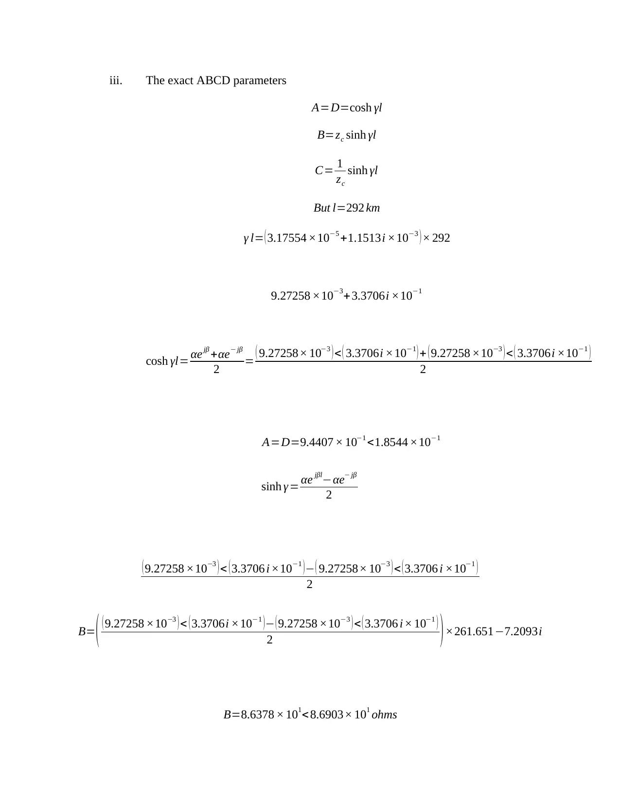
iii. The exact ABCD parameters
A=D=cosh γl
B=zc sinh γl
C= 1
zc
sinh γl
But l=292 km
γ l= ( 3.17554 ×10⁻⁵ +1.1513i ×10−3 ) × 292
9.27258 ×10⁻³+3.3706i ×10−1
cosh γl= αejβ +αe− jβ
2 = ( 9.27258× 10⁻³ ) < ( 3.3706i ×10−1 ) + ( 9.27258 ×10⁻³ ) < ( 3.3706i ×10−1 )
2
A=D=9.4407 × 10⁻¹ <1.8544 ×10⁻¹
sinh γ = αe jβl−αe− jβ
2
( 9.27258 ×10⁻³ ) < ( 3.3706 i ×10−1 ) − ( 9.27258× 10⁻³ ) < ( 3.3706 i ×10−1 )
2
B= ( ( 9.27258 ×10⁻³ ) < ( 3.3706i ×10−1 ) − ( 9.27258 ×10⁻³ ) < ( 3.3706 i× 10−1 )
2 ) ×261.651−7.2093i
B=8.6378 × 101< 8.6903× 101 ohms
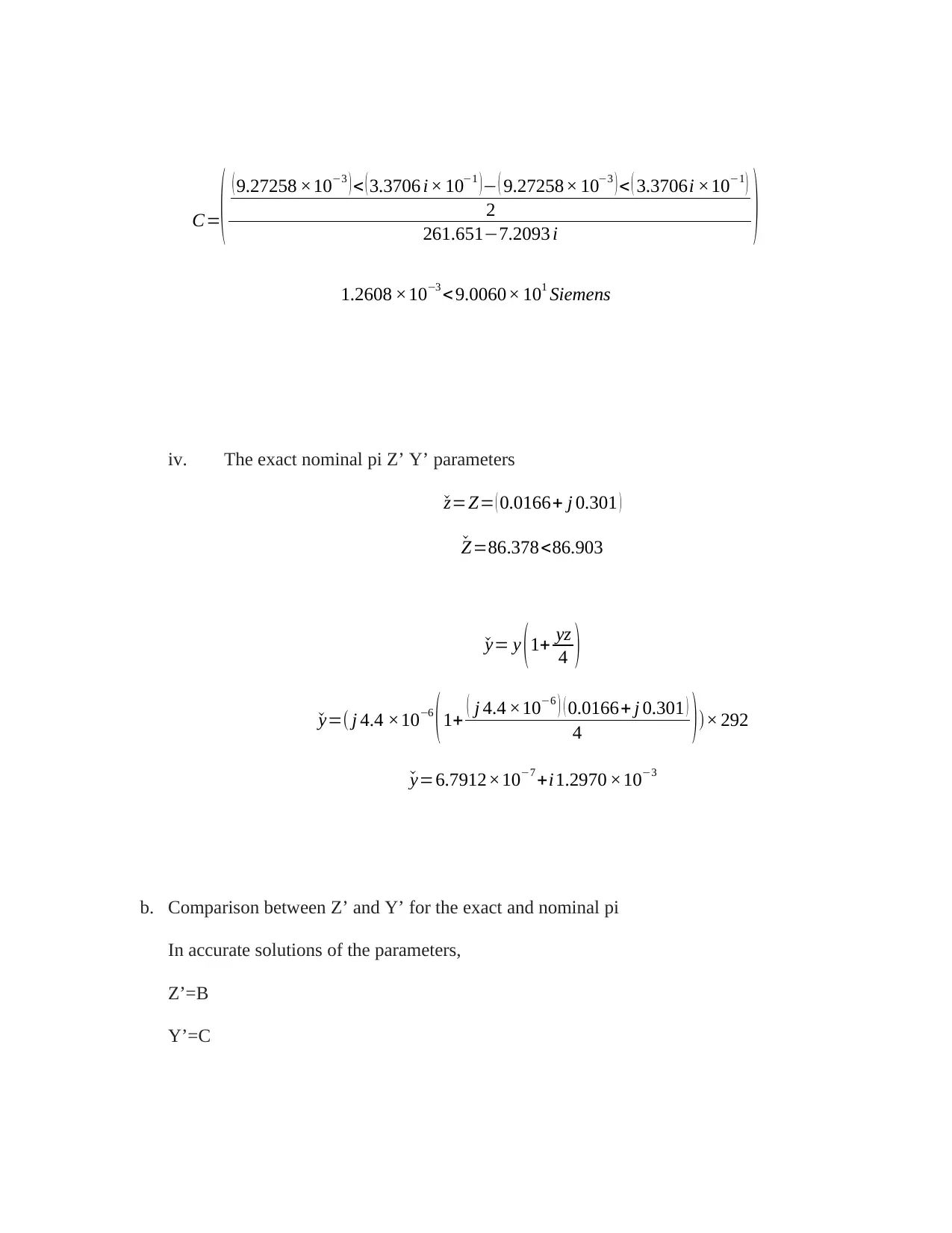
C=( ( 9.27258 ×10⁻³ ) < ( 3.3706 i× 10−1 )− ( 9.27258× 10⁻³ ) < ( 3.3706i ×10−1 )
2
261.651−7.2093 i )
1.2608 ×10⁻³ <9.0060× 101 Siemens
iv. The exact nominal pi Z’ Y’ parameters
ˇz=Z= ( 0.0166+ j 0.301 )
ˇZ=86.378<86.903
ˇy= y (1+ yz
4 )
ˇy=( j 4.4 ×10⁻⁶
(1+ ( j 4.4 ×10⁻⁶ ) ( 0.0166+ j 0.301 )
4 ))× 292
ˇy=6.7912×10⁻⁷ +i1.2970 ×10−3
b. Comparison between Z’ and Y’ for the exact and nominal pi
In accurate solutions of the parameters,
Z’=B
Y’=C
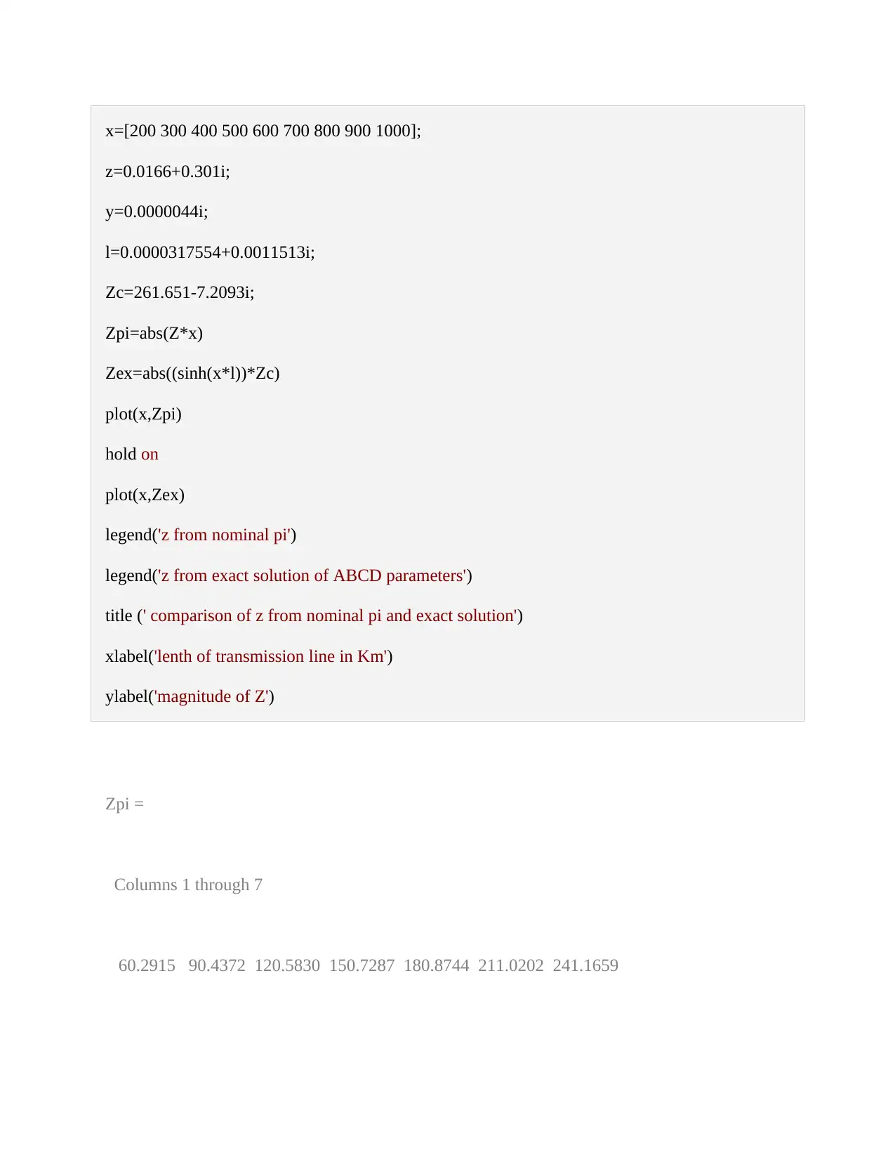
x=[200 300 400 500 600 700 800 900 1000];
z=0.0166+0.301i;
y=0.0000044i;
l=0.0000317554+0.0011513i;
Zc=261.651-7.2093i;
Zpi=abs(Z*x)
Zex=abs((sinh(x*l))*Zc)
plot(x,Zpi)
hold on
plot(x,Zex)
legend('z from nominal pi')
legend('z from exact solution of ABCD parameters')
title (' comparison of z from nominal pi and exact solution')
xlabel('lenth of transmission line in Km')
ylabel('magnitude of Z')
Zpi =
Columns 1 through 7
60.2915 90.4372 120.5830 150.7287 180.8744 211.0202 241.1659
Secure Best Marks with AI Grader
Need help grading? Try our AI Grader for instant feedback on your assignments.
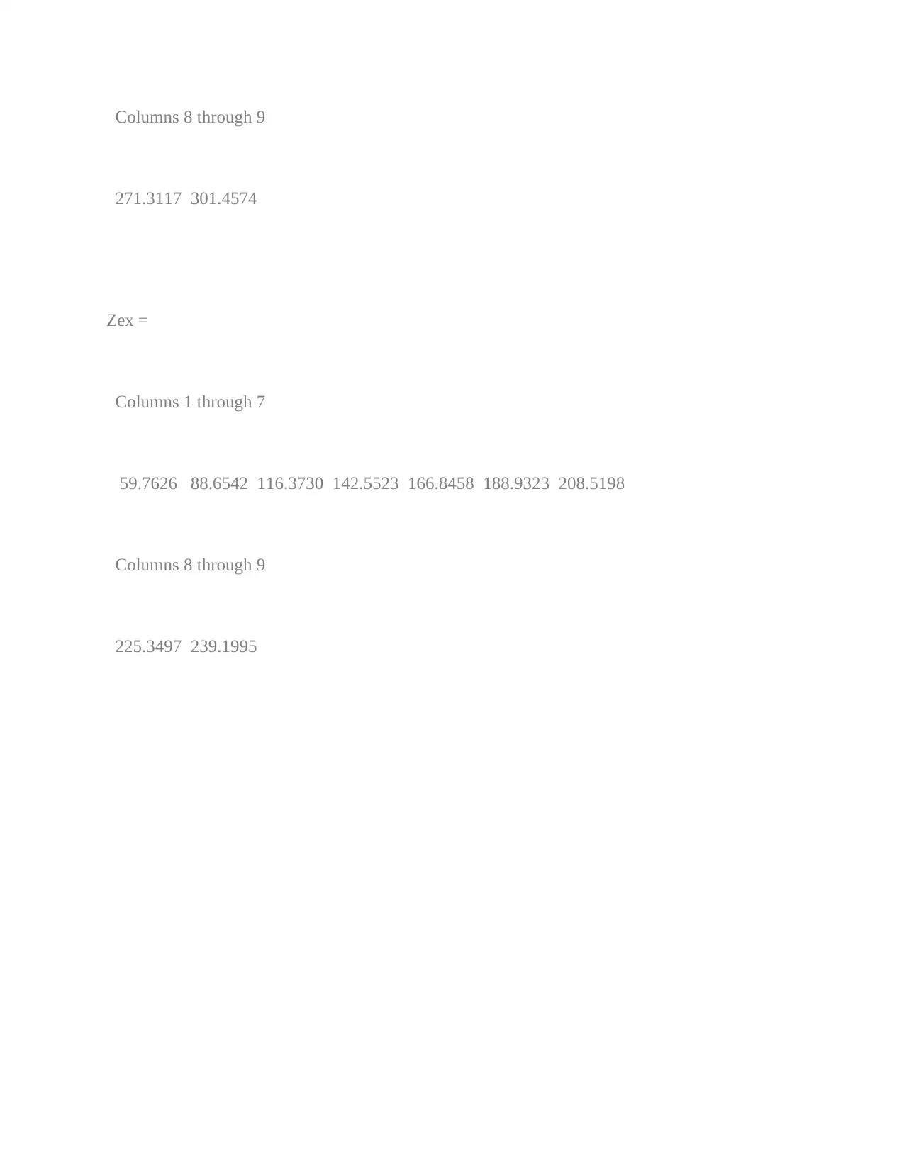
Columns 8 through 9
271.3117 301.4574
Zex =
Columns 1 through 7
59.7626 88.6542 116.3730 142.5523 166.8458 188.9323 208.5198
Columns 8 through 9
225.3497 239.1995
271.3117 301.4574
Zex =
Columns 1 through 7
59.7626 88.6542 116.3730 142.5523 166.8458 188.9323 208.5198
Columns 8 through 9
225.3497 239.1995
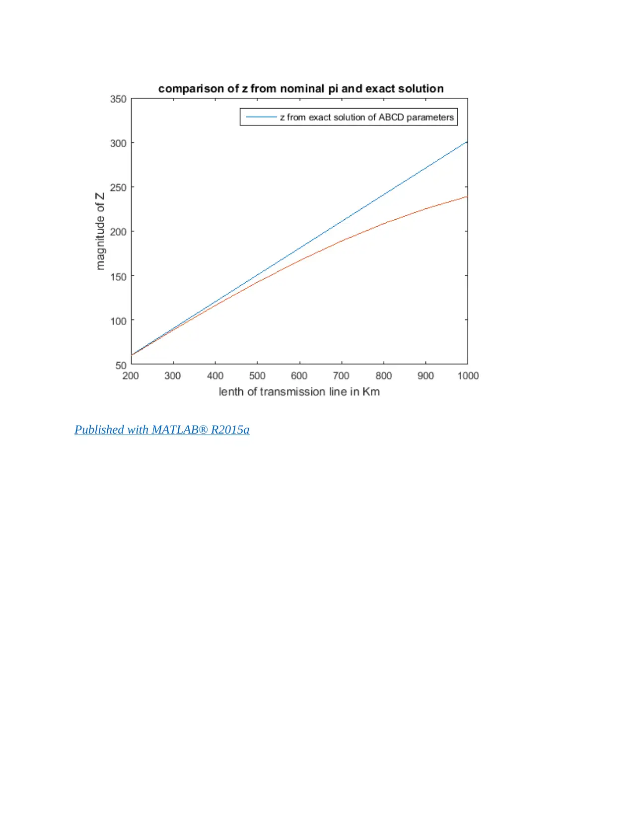
Published with MATLAB® R2015a
lenth of transmission line in Km
200 300 400 500 600 700 800 900 1000
magnitude of Y
10-3
-0.5
0
0.5
1
1.5
2
2.5
3
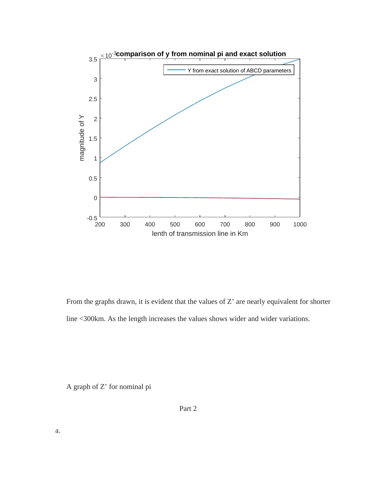
3.5 comparison of y from nominal pi and exact solution
Y from exact solution of ABCD parameters
From the graphs drawn, it is evident that the values of Z’ are nearly equivalent for shorter
line <300km. As the length increases the values shows wider and wider variations.
A graph of Z’ for nominal pi
Part 2
a.
200 300 400 500 600 700 800 900 1000
magnitude of Y
10-3
-0.5
0
0.5
1
1.5
2
2.5
3
3.5 comparison of y from nominal pi and exact solution
Y from exact solution of ABCD parameters
From the graphs drawn, it is evident that the values of Z’ are nearly equivalent for shorter
line <300km. As the length increases the values shows wider and wider variations.
A graph of Z’ for nominal pi
Part 2
a.
Paraphrase This Document
Need a fresh take? Get an instant paraphrase of this document with our AI Paraphraser
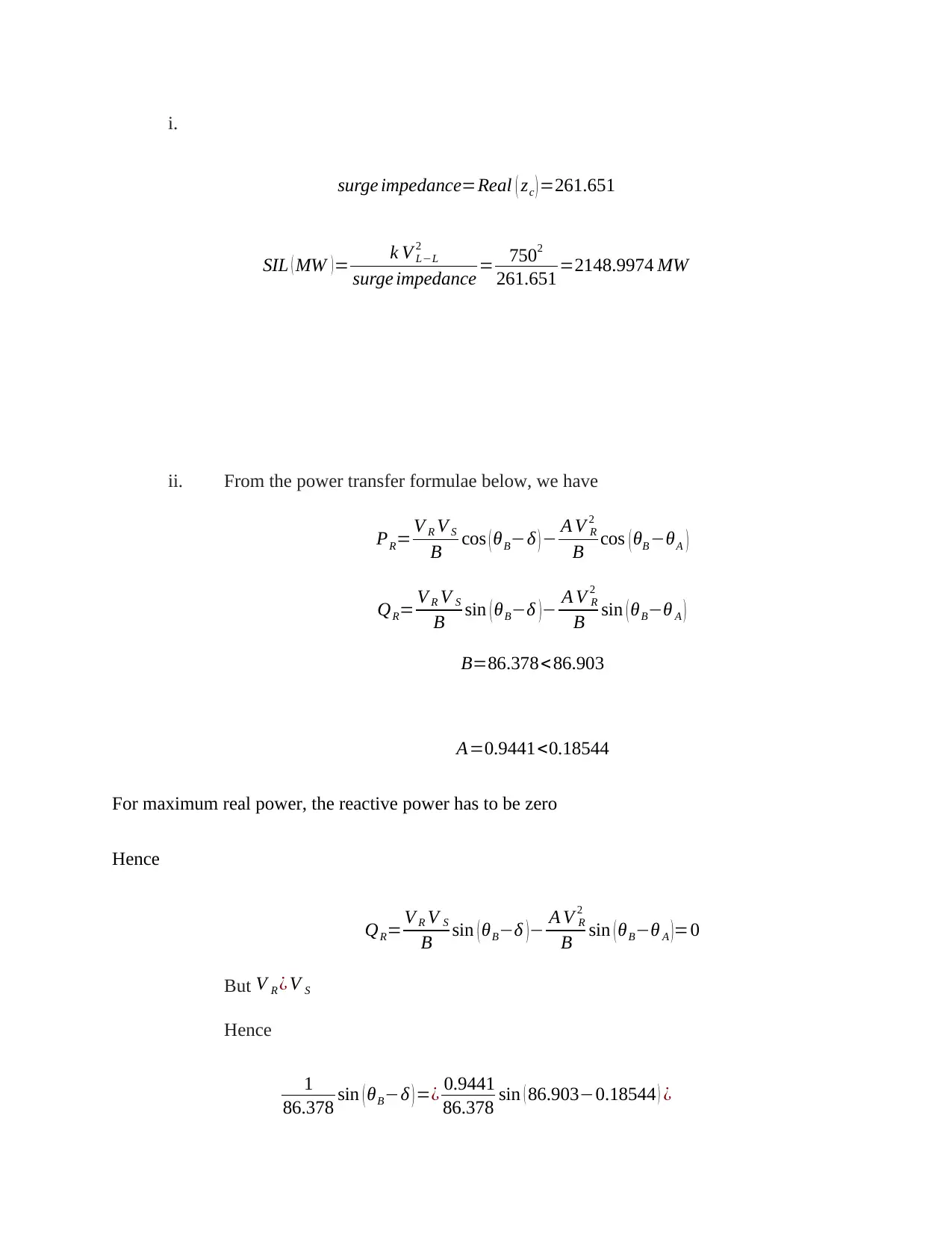
i.
surge impedance=Real ( zc ) =261.651
SIL ( MW ) = k V L−L
2
surge impedance = 7502
261.651 =2148.9974 MW
ii. From the power transfer formulae below, we have
PR= V R V S
B cos ( θB−δ ) − A V R
2
B cos ( θB −θA )
QR= V R V S
B sin ( θB−δ )− A V R
2
B sin ( θB−θ A )
B=86.378<86.903
A=0.9441<0.18544
For maximum real power, the reactive power has to be zero
Hence
QR= V R V S
B sin ( θB−δ )− A V R
2
B sin (θB−θ A )=0
But V R ¿ V S
Hence
1
86.378 sin ( θB−δ ) =¿ 0.9441
86.378 sin ( 86.903−0.18544 ) ¿
sin ( θB−δ ) =¿ 0.94255 ¿
( θB−δ ) =70.4845
Substituting the value of ( θB−δ ) in the real part of the equation, we get
PR= 750× 750
86.378 cos 70.4845− 0.9441×7502
86.378 cos ( 86.7176 )
1823.415 MW
As a percentage of SIL,
1823.415 MW
2148.9974 MW × 100=84.84955%
b. When the transmission line is operated at 500kV,
V R ¿ V S=500 kV
SIL ( MW )= k V L−L
2
surge impedance = 5002
261.651 =955.4712 MW
¿ 955.4712 MW
Maximum real power loading
Since
V R ¿ V S
From part b,
1
86.378 sin ( θB−δ ) =¿ 0.9441
86.378 sin ( 86.903−0.18544 ) ¿
sin ( θB−δ ) =¿ 0.94255 ¿
( θB−δ ) =70.4845
Substituting, we obtain
PR= 500× 500
86.378 cos 70.4845− 0.9441×5002
86.378 cos ( 86.7176 )
810.4065 MW
Part 3
a.
i.
PR= V R V S
B cos ( θB−δ ) − A V R
2
B cos ( θB −θA )
QR= V R V S
B sin ( θB−δ )− A V R
2
B sin ( θB−θ A )
V S =Vbase ×Vspu=1.02× 750=765 kv
V R=Vbase × Vspu=0.98 ×750=735 kv
δ =δmax=36
Secure Best Marks with AI Grader
Need help grading? Try our AI Grader for instant feedback on your assignments.
PR= 765× 735
86.378 cos (86.903−36)− 0.9441×7352
86.378 cos ( 86.7176 )
3768.9270 MW
SIL ( MW ) = k V L−L
2
surge impedance = 7502
261.651 =2148.9974 MW
As a percentage of SIL,
3768.9270
2148.9974 MW × 100=175.3381 %
b.
Vbase=500 kv
V S =Vbase ×Vspu=1.02× 500=510 kv
V R=Vbase × Vspu=0.98 ×500=490 kv
From part a, we have
PR= V R V S
B cos ( θB−δ ) − A V R
2
B cos ( θB −θA )
QR= V R V S
B sin ( θB−δ )− A V R
2
B sin ( θB−θ A )
PR= 510× 490
86.378 cos(86.903−36)− 0.9441 ×4902
86.378 cos ( 86.7176 )
Practical loadability 1674.2310 MW
Part 4
i.
V s =AV R + B I R
V R=Vbase × VRpu=750× 0.96=729 kv
V R=720 KV < 0
I R =1.90 KA <0
A=0.9441<0.18544
B=86.378<86.903
Substituting the variables in the equation, we get
V s =((0.9441<0.18544)720<0)+( ( 86.378< 86.903 ) (1.90< 0 ) )
708.3593<13.5595 KV
ii. Under no load,
I R =0
V s =AV R
V R=¿ 708.3593 <13.5595
(0.9441<0.18544) ¿
V NL=751.8252<13.3387
iii.
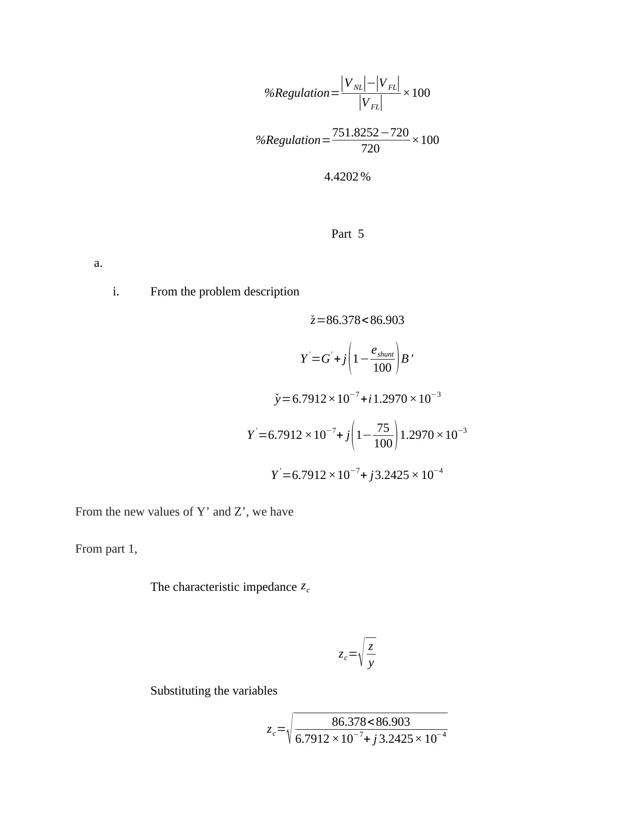
%Regulation=
|V NL|−|V FL|
|V FL| ×100
%Regulation=751.8252−720
720 ×100
4.4202 %
Part 5
a.
i. From the problem description
ˇz=86.378< 86.903
Y '=G' + j (1− eshunt
100 )B '
ˇy=6.7912×10⁻⁷ +i1.2970 ×10−3
Y ' =6.7912 ×10⁻⁷+ j ( 1− 75
100 ) 1.2970 ×10⁻³
Y ' =6.7912 ×10⁻⁷+ j3.2425 × 10−4
From the new values of Y’ and Z’, we have
From part 1,
The characteristic impedance zc
zc= √ z
y
Substituting the variables
zc= √ 86.378<86.903
6.7912 ×10⁻⁷+ j 3.2425× 10⁻⁴
Paraphrase This Document
Need a fresh take? Get an instant paraphrase of this document with our AI Paraphraser
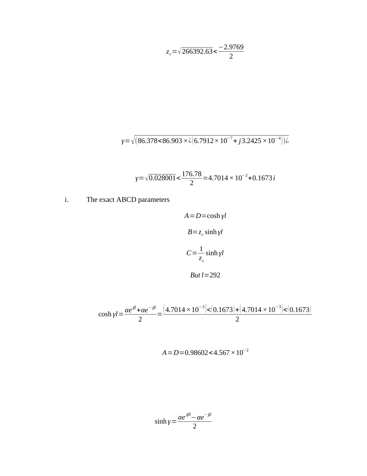
zc= √266392.63< −2.9769
2
γ= √(86.378<86.903 ׿ ( 6.7912× 10⁻⁷ + j3.2425 ×10−4 ) )¿
γ= √0.028001< 176.78
2 =4.7014 × 10⁻³ +0.1673 i
i. The exact ABCD parameters
A=D=cosh γl
B=zc sinh γl
C= 1
zc
sinh γl
But l=292
cosh γl= αejβ +αe− jβ
2 = ( 4.7014 ×10⁻³ )< ( 0.1673 ) + ( 4.7014 ×10⁻³ )< ( 0.1673 )
2
A=D=0.98602<4.567 ×10⁻²
sinh γ = αe jβl−αe− jβ
2
2
γ= √(86.378<86.903 ׿ ( 6.7912× 10⁻⁷ + j3.2425 ×10−4 ) )¿
γ= √0.028001< 176.78
2 =4.7014 × 10⁻³ +0.1673 i
i. The exact ABCD parameters
A=D=cosh γl
B=zc sinh γl
C= 1
zc
sinh γl
But l=292
cosh γl= αejβ +αe− jβ
2 = ( 4.7014 ×10⁻³ )< ( 0.1673 ) + ( 4.7014 ×10⁻³ )< ( 0.1673 )
2
A=D=0.98602<4.567 ×10⁻²
sinh γ = αe jβl−αe− jβ
2
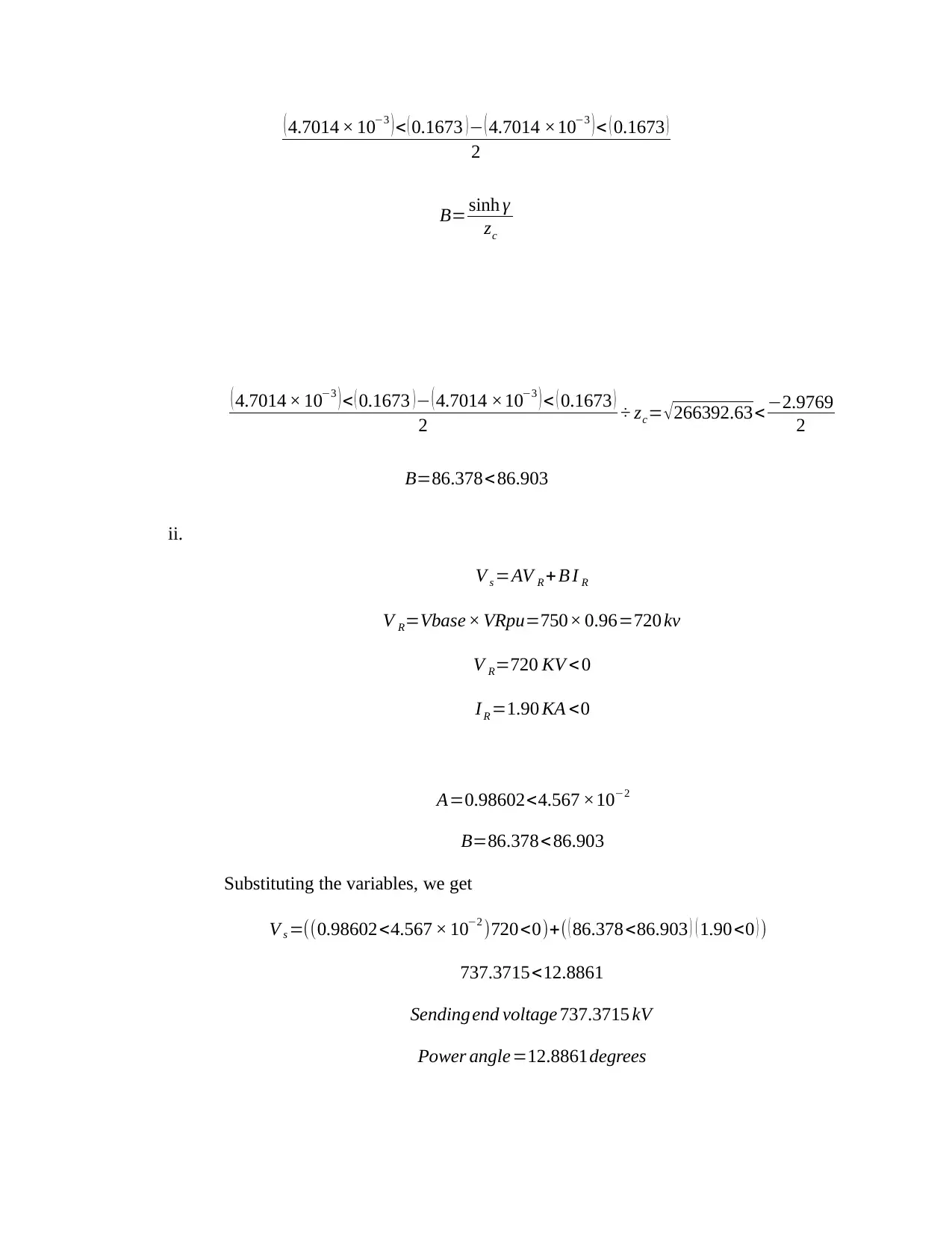
( 4.7014 × 10⁻³ ) < ( 0.1673 )− ( 4.7014 ×10⁻³ ) < ( 0.1673 )
2
B= sinh γ
zc
( 4.7014 × 10⁻³ ) < ( 0.1673 )− ( 4.7014 ×10⁻³ ) < ( 0.1673 )
2 ÷ zc= √266392.63<−2.9769
2
B=86.378<86.903
ii.
V s =AV R + B I R
V R=Vbase × VRpu=750× 0.96=720 kv
V R=720 KV < 0
I R =1.90 KA <0
A=0.98602<4.567 ×10⁻²
B=86.378<86.903
Substituting the variables, we get
V s =((0.98602<4.567 × 10⁻² )720<0)+( ( 86.378<86.903 ) ( 1.90<0 ) )
737.3715<12.8861
Sending end voltage 737.3715 kV
Power angle=12.8861degrees
2
B= sinh γ
zc
( 4.7014 × 10⁻³ ) < ( 0.1673 )− ( 4.7014 ×10⁻³ ) < ( 0.1673 )
2 ÷ zc= √266392.63<−2.9769
2
B=86.378<86.903
ii.
V s =AV R + B I R
V R=Vbase × VRpu=750× 0.96=720 kv
V R=720 KV < 0
I R =1.90 KA <0
A=0.98602<4.567 ×10⁻²
B=86.378<86.903
Substituting the variables, we get
V s =((0.98602<4.567 × 10⁻² )720<0)+( ( 86.378<86.903 ) ( 1.90<0 ) )
737.3715<12.8861
Sending end voltage 737.3715 kV
Power angle=12.8861degrees
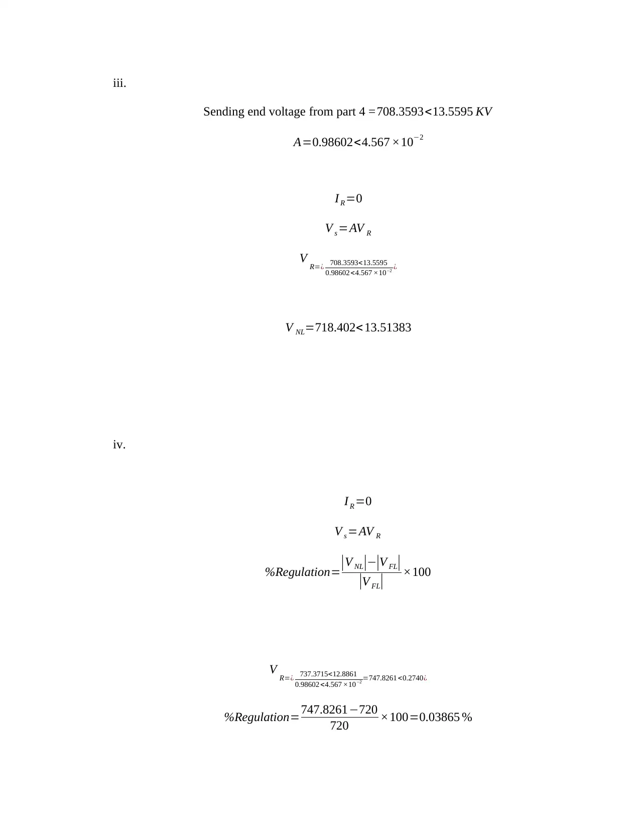
iii.
Sending end voltage from part 4 = 708.3593<13.5595 KV
A=0.98602<4.567 ×10⁻²
I R =0
V s =AV R
V R=¿ 708.3593<13.5595
0.98602<4.567 ×10⁻² ¿
V NL=718.402<13.51383
iv.
I R =0
V s =AV R
%Regulation=
|V NL|−|V FL|
|V FL| ×100
V R=¿ 737.3715<12.8861
0.98602 <4.567 ×10−2 =747.8261 <0.2740¿
%Regulation=747.8261−720
720 ×100=0.03865 %
Secure Best Marks with AI Grader
Need help grading? Try our AI Grader for instant feedback on your assignments.
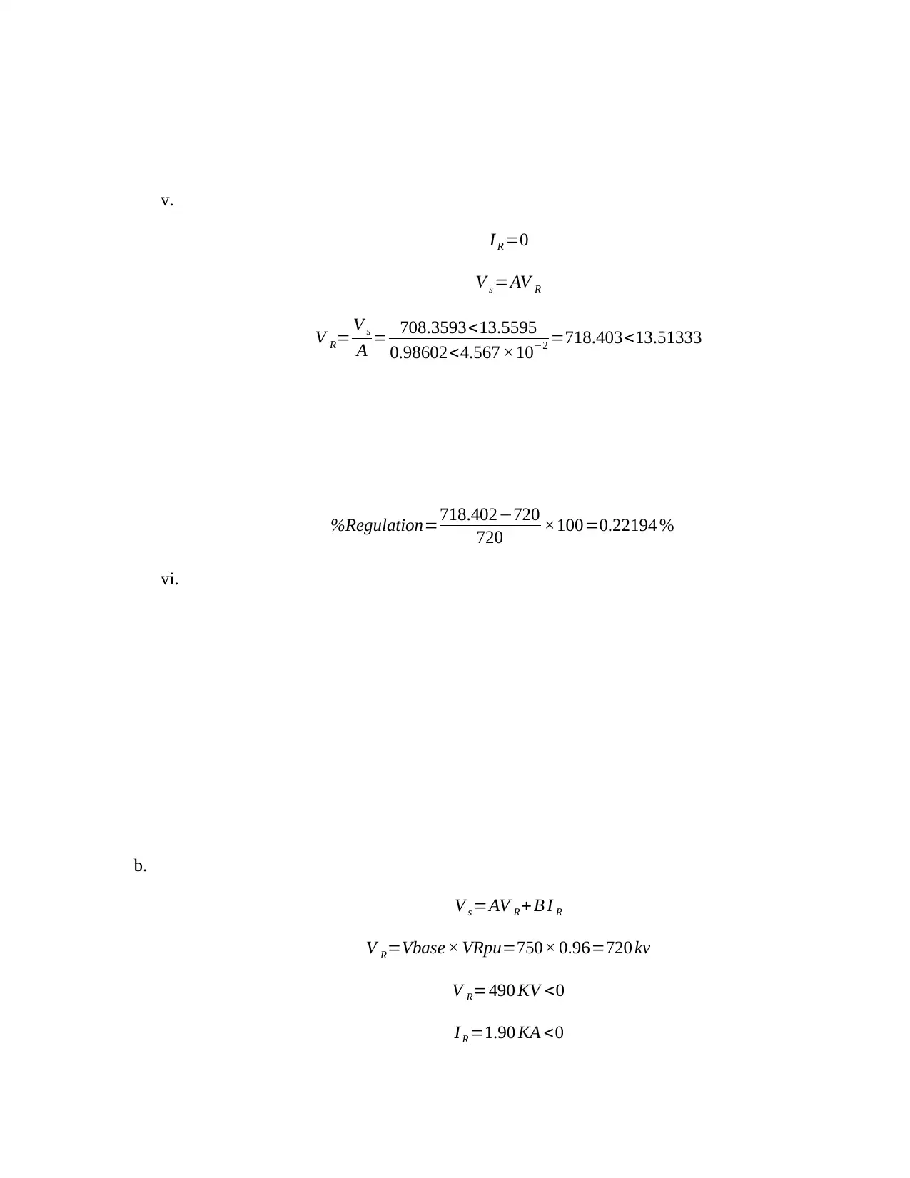
v.
I R =0
V s =AV R
V R= V s
A = 708.3593<13.5595
0.98602<4.567 ×10−2 =718.403<13.51333
%Regulation=718.402−720
720 ×100=0.22194 %
vi.
b.
V s =AV R + B I R
V R=Vbase × VRpu=750× 0.96=720 kv
V R=490 KV <0
I R =1.90 KA <0
I R =0
V s =AV R
V R= V s
A = 708.3593<13.5595
0.98602<4.567 ×10−2 =718.403<13.51333
%Regulation=718.402−720
720 ×100=0.22194 %
vi.
b.
V s =AV R + B I R
V R=Vbase × VRpu=750× 0.96=720 kv
V R=490 KV <0
I R =1.90 KA <0
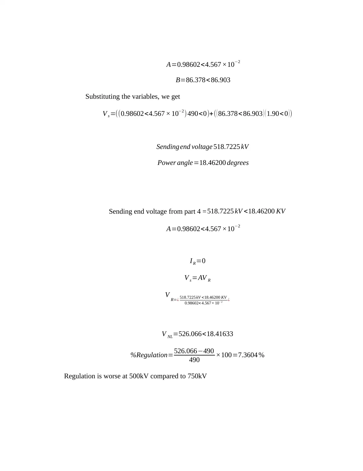
A=0.98602<4.567 ×10⁻²
B=86.378<86.903
Substituting the variables, we get
V s =((0.98602<4.567 × 10⁻² ) 490<0)+( ( 86.378<86.903 ) ( 1.90< 0 ) )
Sending end voltage 518.7225 kV
Power angle=18.46200 degrees
Sending end voltage from part 4 =518.7225 kV <18.46200 KV
A=0.98602<4.567 ×10⁻²
I R =0
V s =AV R
V R=¿ 518.7225 kV <18.46200 KV
0.98602< 4.567× 10⁻² ¿
V NL=526.066<18.41633
%Regulation=526.066−490
490 ×100=7.3604 %
Regulation is worse at 500kV compared to 750kV
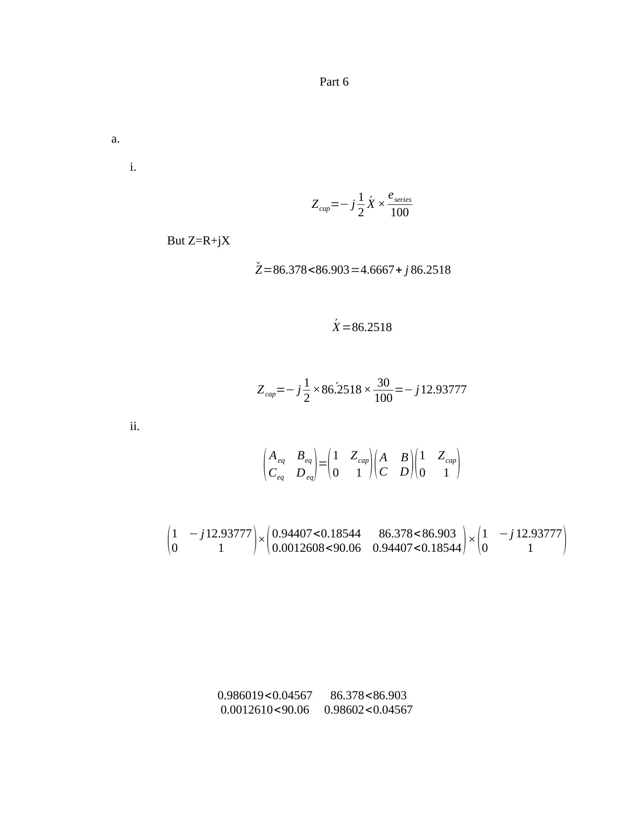
Part 6
a.
i.
Zcap=− j 1
2 ´X × eseries
100
But Z=R+jX
ˇZ=86.378<86.903=4.6667+ j 86.2518
´X =86.2518
Zcap=− j 1
2 ´×86.2518 × 30
100 =− j12.93777
ii.
( Aeq Beq
Ceq Deq
)=(1 Zcap
0 1 ) ( A B
C D ) (1 Zcap
0 1 )
(1 − j12.93777
0 1 )× (0.94407<0.18544 86.378< 86.903
0.0012608<90.06 0.94407<0.18544 )× (1 − j 12.93777
0 1 )
0.986019<0.04567 86.378<86.903
0.0012610<90.06 0.98602<0.04567
Paraphrase This Document
Need a fresh take? Get an instant paraphrase of this document with our AI Paraphraser
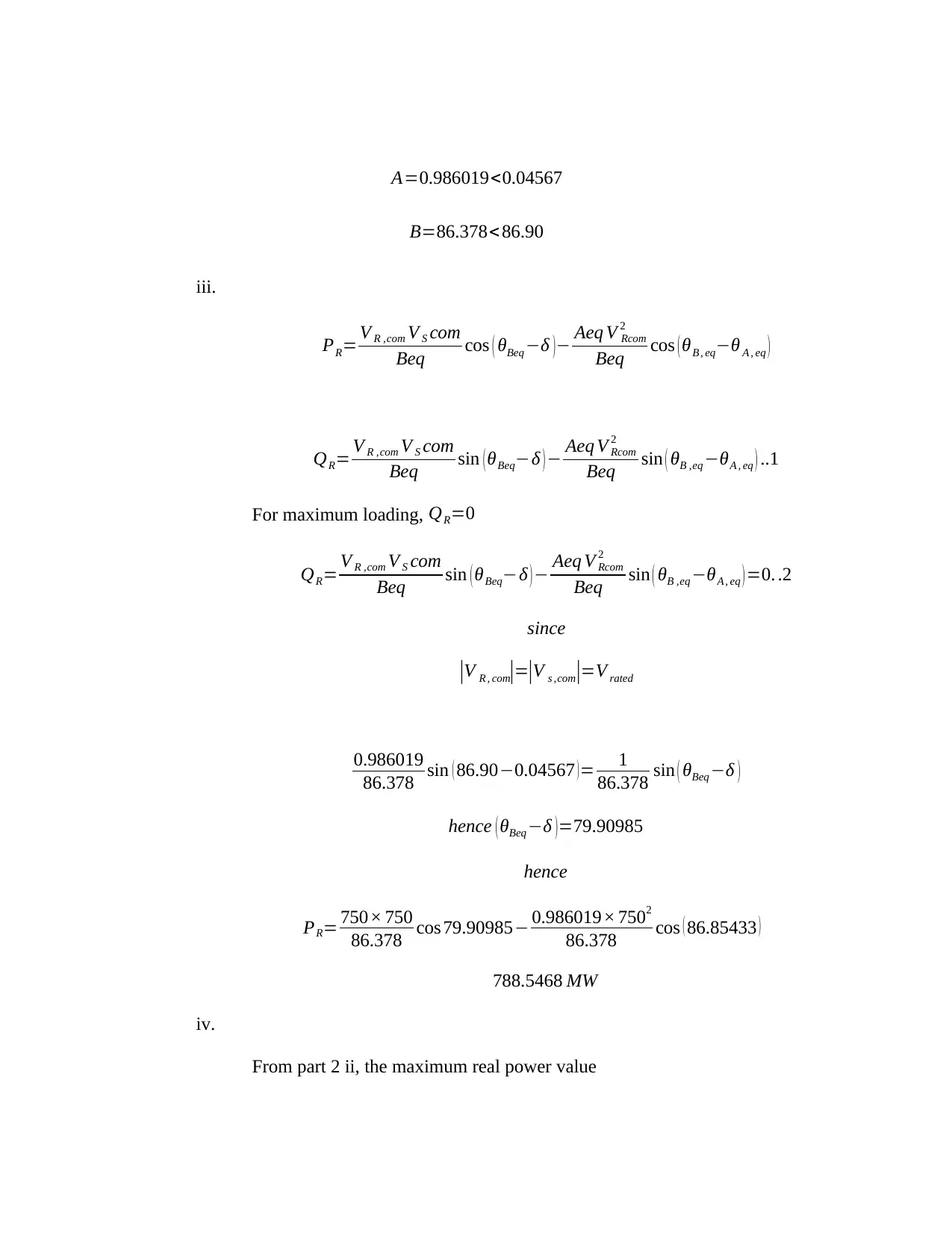
A=0.986019<0.04567
B=86.378< 86.90
iii.
PR= V R ,com V S com
Beq cos ( θBeq −δ )− Aeq V Rcom
2
Beq cos ( θB , eq−θ A , eq )
QR= V R ,com V S com
Beq sin ( θBeq−δ ) − Aeq V Rcom
2
Beq sin ( θB ,eq −θA , eq ) ..1
For maximum loading, QR=0
QR= V R ,com V S com
Beq sin ( θBeq−δ ) − Aeq V Rcom
2
Beq sin ( θB ,eq −θA , eq ) =0. .2
since
|V R , com|=|V s ,com|=V rated
0.986019
86.378 sin ( 86.90−0.04567 ) = 1
86.378 sin ( θBeq −δ )
hence ( θBeq −δ )=79.90985
hence
PR= 750× 750
86.378 cos 79.90985− 0.986019× 7502
86.378 cos ( 86.85433 )
788.5468 MW
iv.
From part 2 ii, the maximum real power value
PR=1823.415 MW
From part 6 iii, we have
PR=788.5468 MW
The difference =1823.415 MW −788.5468 MW =1034.8682 MW
As per percentage of the difference in maximum power of SIL, we have
1034.8682 MW
2148.9974 MW × 100=48.1559 %
v.
PR= V R V S
B cos ( θB−δ ) − A V R
2
B cos ( θB −θA )
QR= V R V S
B sin ( θB−δ )− A V R
2
B sin (θB−θ A )
V S =Vbase ×Vspu=1.02× 750=765 kv
V R=Vbase × Vspu=0.98 ×750=735 kv
δ=δmax=36
PR= 765× 735
86.378 cos (86.90−36)− 0.986019× 7352
86.378 cos ( 86.85433 )
PR=3766.966194 MW
vi.
The difference between the practical maximum real power delivery values of
the uncompensated transmission line of part 3a and the compensated
transmission
From part 3a,
PR=3768.9270 MW
From 6 v,
PR=3766.966194 MW
The difference = PR=3766.966194 MW −3766.966194 MW =1.960806 MW
Expressed as percentage of SIL,
1.960806 MW
2148.9974 MW × 100=0.0912%
b.
From par 6 a v, we have the receiving end power relations as
PR= V R V S
B cos ( θB−δ ) − A V R
2
B cos ( θB −θA )
QR= V R V S
B sin ( θB−δ )− A V R
2
B sin (θB−θ A )
V S =Vbase ×Vspu=1.02× 500=510 kv
V R=Vbase × Vspu=0.98 ×500=490 kv
δ=δmax=36
1 out of 22


Your All-in-One AI-Powered Toolkit for Academic Success.
+13062052269
info@desklib.com
Available 24*7 on WhatsApp / Email
![[object Object]](/_next/static/media/star-bottom.7253800d.svg)
Unlock your academic potential
© 2024 | Zucol Services PVT LTD | All rights reserved.