Quantitative Analysis .
VerifiedAdded on 2023/05/29
|10
|2223
|84
AI Summary
This article discusses quantitative analysis in business statistics, including probability, binomial distribution, hypothesis testing, and more. It also explores the applications of statistics in financial analysis, production tracking, and planning efficiency. The article provides expert guidance on the topic.
Contribute Materials
Your contribution can guide someone’s learning journey. Share your
documents today.

Running head: Quantitative Analysis
Quantitative Analysis
Student Name
Institution Name
Date of Submission
1
Quantitative Analysis
Student Name
Institution Name
Date of Submission
1
Secure Best Marks with AI Grader
Need help grading? Try our AI Grader for instant feedback on your assignments.
Quantitative Analysis
Introduction
Business statistics can be defined as a branch of statics that is applied to help ease business
activities. The statistics is helpful in ensuring quality assurance in business. In addition,
statistics allows for efficient financial analysis, production tracking and planning efficiency
as well as several areas of business production (Morien, 2007). the general statistics is dived
in two broad categories that is the descriptive and the inferential. Descriptive is applicable in
explaining numbers while the inferential is applied to infer relationships from the parameters
of the population.
Inferential statistics are more useful in cases where the business managers have limited data.
For instance, the sampling, probability and models are useful for predicting future trends.
Areas such as marketing largely depend on the inferential statistics due to the inability to
involve the entire population in the research (Wegner, 2010). So as to gauge the future
business budget requirements, the finance department usually applies statistical models to try
represent a future occurrence.
Being that several business data come in form of numbers, descriptive statistics is a useful
tool when it comes to breaking down such data. Statistical variables such as the mean,
median and mode can assist the management monitor the prevailing activities as well as make
informed business judgements (Nick, 2007). The use of ratios is occasionally applied to assist
give highlight of the big picture.
Task 1: Selecting the random sample and creating the sample data file
The data to be statistically analysed composed of information about 400 people from a survey
done in a unique State in the USA within a specific year. This population is comprised of
working individuals who were drawing wages as at the time of the survey.
Before commencing the data analysis 50 random individual ID’s will be selected and the
sample used for the purpose of the analysis. The sampling method will be without
replacement where individual ID’s will only be selected once.
Definition of the variables;
V1: Wage
V2: Occupation
V3: Age
Quantitative Analysis
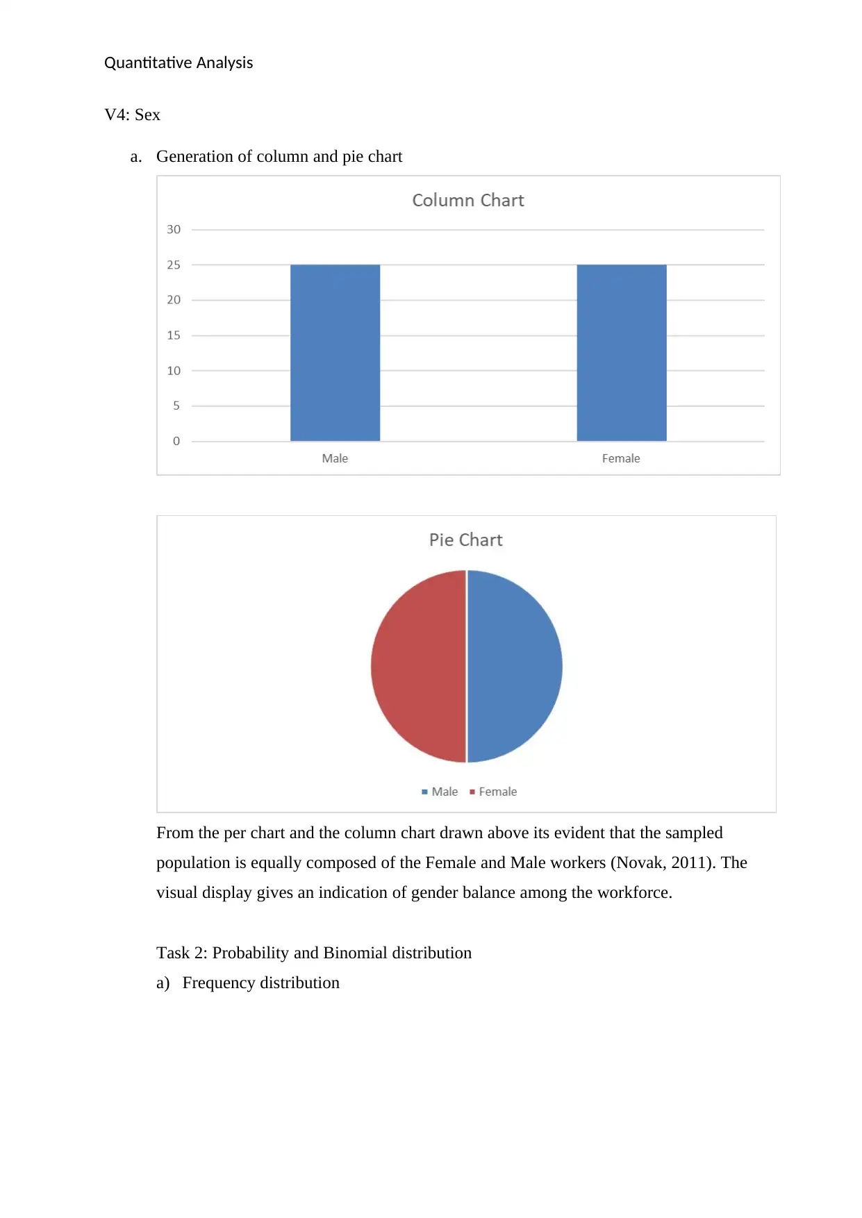
V4: Sex
a. Generation of column and pie chart
From the per chart and the column chart drawn above its evident that the sampled
population is equally composed of the Female and Male workers (Novak, 2011). The
visual display gives an indication of gender balance among the workforce.
Task 2: Probability and Binomial distribution
a) Frequency distribution
Quantitative Analysis
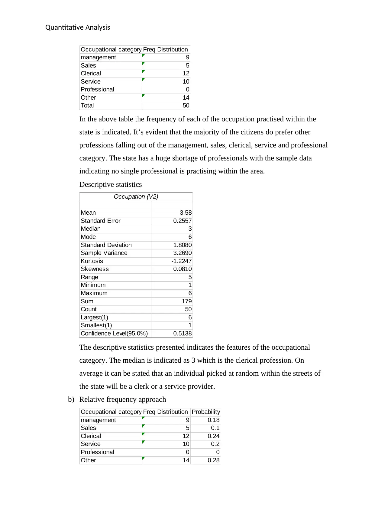
Occupational category Freq Distribution
management 9
Sales 5
Clerical 12
Service 10
Professional 0
Other 14
Total 50
In the above table the frequency of each of the occupation practised within the
state is indicated. It’s evident that the majority of the citizens do prefer other
professions falling out of the management, sales, clerical, service and professional
category. The state has a huge shortage of professionals with the sample data
indicating no single professional is practising within the area.
Descriptive statistics
Occupation (V2)
Mean 3.58
Standard Error 0.2557
Median 3
Mode 6
Standard Deviation 1.8080
Sample Variance 3.2690
Kurtosis -1.2247
Skewness 0.0810
Range 5
Minimum 1
Maximum 6
Sum 179
Count 50
Largest(1) 6
Smallest(1) 1
Confidence Level(95.0%) 0.5138
The descriptive statistics presented indicates the features of the occupational
category. The median is indicated as 3 which is the clerical profession. On
average it can be stated that an individual picked at random within the streets of
the state will be a clerk or a service provider.
b) Relative frequency approach
Occupational category Freq Distribution Probability
management 9 0.18
Sales 5 0.1
Clerical 12 0.24
Service 10 0.2
Professional 0 0
Other 14 0.28
Secure Best Marks with AI Grader
Need help grading? Try our AI Grader for instant feedback on your assignments.
Quantitative Analysis
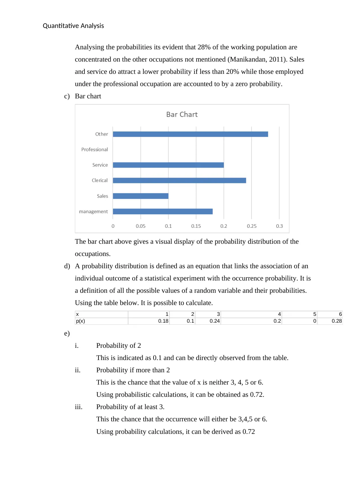
Analysing the probabilities its evident that 28% of the working population are
concentrated on the other occupations not mentioned (Manikandan, 2011). Sales
and service do attract a lower probability if less than 20% while those employed
under the professional occupation are accounted to by a zero probability.
c) Bar chart
The bar chart above gives a visual display of the probability distribution of the
occupations.
d) A probability distribution is defined as an equation that links the association of an
individual outcome of a statistical experiment with the occurrence probability. It is
a definition of all the possible values of a random variable and their probabilities.
Using the table below. It is possible to calculate.
x 1 2 3 4 5 6
p(x) 0.18 0.1 0.24 0.2 0 0.28
e)
i. Probability of 2
This is indicated as 0.1 and can be directly observed from the table.
ii. Probability if more than 2
This is the chance that the value of x is neither 3, 4, 5 or 6.
Using probabilistic calculations, it can be obtained as 0.72.
iii. Probability of at least 3.
This the chance that the occurrence will either be 3,4,5 or 6.
Using probability calculations, it can be derived as 0.72
Quantitative Analysis
f) Using the prior information available from the previous research and the
calculated probabilities it is possible to obtain posterior probabilities and
calculate:
i. Probability if exactly two.
Through the excel calculations this is obtained as 0.1.
ii. Probability of less than 2
The posterior probability is obtained as 0.18.
iii. Probability if at least 6. This gives the chance that the value is either 6 or
above. From the calculations it is obtained as 0.28.
Task 3: Estimation and hypothesis testing
This is the application of statistics to obtain the chance that a given probability’s truth value
is true. This process is usually characterised by four steps;
Formulation of null hypothesis; This is stated as H0, is the indication that
the observed features are due to pure chance and have no statistical
relevance. On the other hand, the alternative hypothesis indicated as Ha,
this is the chance that the observations indicate a real effect combined with
a component of chance variation.
Identification of test statistic, this is the value that is applied in testing the
truth value of the null hypothesis.
Computation of the p_value, this is the probability that a test statistic at
least as significant as the one observed will be obtained should the null
hypothesis be true. A smaller p_value indicates a stronger evidence against
the null hypothesis.
Comparison of the p_value to the identified significance value α. The
decision criteria is that should the value of p be less or equals to α, then
the observed statistical effect is said to be significant (Sotos, Vanhoof,
Noortgate, & Onghena, 2009). This way the null hypothesis is ruled
a. Drawing the histogram
Histogram can be defined as an efficient representation of a numerical data’s
distribution. The construction of a histogram involves first classifying the data in to
Quantitative Analysis
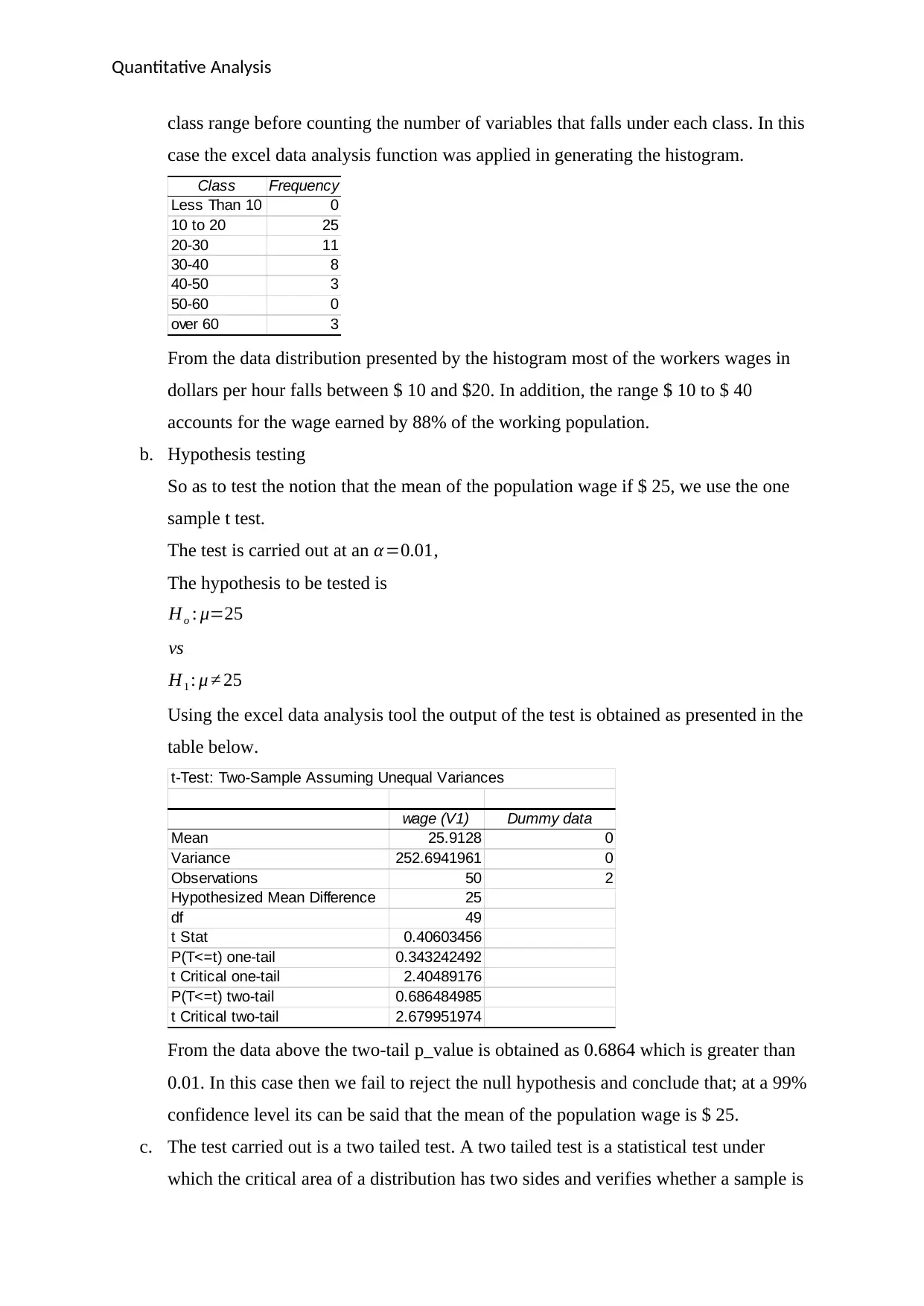
class range before counting the number of variables that falls under each class. In this
case the excel data analysis function was applied in generating the histogram.
Class Frequency
Less Than 10 0
10 to 20 25
20-30 11
30-40 8
40-50 3
50-60 0
over 60 3
From the data distribution presented by the histogram most of the workers wages in
dollars per hour falls between $ 10 and $20. In addition, the range $ 10 to $ 40
accounts for the wage earned by 88% of the working population.
b. Hypothesis testing
So as to test the notion that the mean of the population wage if $ 25, we use the one
sample t test.
The test is carried out at an α =0.01,
The hypothesis to be tested is
Ho : μ=25
vs
H1 : μ ≠ 25
Using the excel data analysis tool the output of the test is obtained as presented in the
table below.
t-Test: Two-Sample Assuming Unequal Variances
wage (V1) Dummy data
Mean 25.9128 0
Variance 252.6941961 0
Observations 50 2
Hypothesized Mean Difference 25
df 49
t Stat 0.40603456
P(T<=t) one-tail 0.343242492
t Critical one-tail 2.40489176
P(T<=t) two-tail 0.686484985
t Critical two-tail 2.679951974
From the data above the two-tail p_value is obtained as 0.6864 which is greater than
0.01. In this case then we fail to reject the null hypothesis and conclude that; at a 99%
confidence level its can be said that the mean of the population wage is $ 25.
c. The test carried out is a two tailed test. A two tailed test is a statistical test under
which the critical area of a distribution has two sides and verifies whether a sample is
Paraphrase This Document
Need a fresh take? Get an instant paraphrase of this document with our AI Paraphraser
Quantitative Analysis
greater than or less than a certain value. In the case above the alternative hypothesis is
accepted should the mean either be less than or greater than 25. This way we can
prove that the test is two tailed.
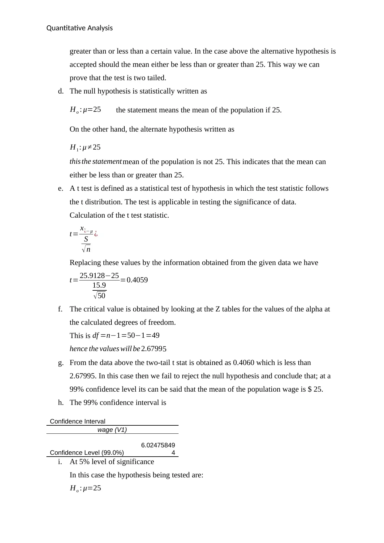
d. The null hypothesis is statistically written as
Ho : μ=25 the statement means the mean of the population if 25.
On the other hand, the alternate hypothesis written as
H1 : μ ≠ 25
this the statement mean of the population is not 25. This indicates that the mean can
either be less than or greater than 25.
e. A t test is defined as a statistical test of hypothesis in which the test statistic follows
the t distribution. The test is applicable in testing the significance of data.
Calculation of the t test statistic.
t= x¯¿− μ
S
√n
¿
Replacing these values by the information obtained from the given data we have
t= 25.9128−25
15.9
√ 50
=0.4059
f. The critical value is obtained by looking at the Z tables for the values of the alpha at
the calculated degrees of freedom.
This is df =n−1=50−1=49
hence the values will be 2.67995
g. From the data above the two-tail t stat is obtained as 0.4060 which is less than
2.67995. In this case then we fail to reject the null hypothesis and conclude that; at a
99% confidence level its can be said that the mean of the population wage is $ 25.
h. The 99% confidence interval is
Confidence Interval
wage (V1)
Confidence Level (99.0%)
6.02475849
4
i. At 5% level of significance
In this case the hypothesis being tested are:
Ho : μ=25
greater than or less than a certain value. In the case above the alternative hypothesis is
accepted should the mean either be less than or greater than 25. This way we can
prove that the test is two tailed.
d. The null hypothesis is statistically written as
Ho : μ=25 the statement means the mean of the population if 25.
On the other hand, the alternate hypothesis written as
H1 : μ ≠ 25
this the statement mean of the population is not 25. This indicates that the mean can
either be less than or greater than 25.
e. A t test is defined as a statistical test of hypothesis in which the test statistic follows
the t distribution. The test is applicable in testing the significance of data.
Calculation of the t test statistic.
t= x¯¿− μ
S
√n
¿
Replacing these values by the information obtained from the given data we have
t= 25.9128−25
15.9
√ 50
=0.4059
f. The critical value is obtained by looking at the Z tables for the values of the alpha at
the calculated degrees of freedom.
This is df =n−1=50−1=49
hence the values will be 2.67995
g. From the data above the two-tail t stat is obtained as 0.4060 which is less than
2.67995. In this case then we fail to reject the null hypothesis and conclude that; at a
99% confidence level its can be said that the mean of the population wage is $ 25.
h. The 99% confidence interval is
Confidence Interval
wage (V1)
Confidence Level (99.0%)
6.02475849
4
i. At 5% level of significance
In this case the hypothesis being tested are:
Ho : μ=25

Quantitative Analysis
vs
H1 : μ>25
This is a one tail test.
Test hypotheis at 5% level of significance
t-Test: Two-Sample Assuming Unequal Variances
wage (V1) Dummy data
Mean 25.9128 0
Variance 252.6941961 0
Observations 50 2
Hypothesized Mean Difference 25
df 49
t Stat 0.40603456
P(T<=t) one-tail 0.343242492
t Critical one-tail 1.676550893
P(T<=t) two-tail 0.686484985
t Critical two-tail 2.009575237
Being that the one tail p_value is greater than 0.05, we fail to reject the null
hypothesis and conclude that the population mean is 25.
j. Considering the critical value, its is observed that t Critical One tail is 1.67655 which
is greater than the t Stat, we thereby fail to reject the null hypothesis.
k. Finding the 95% confidence interval
95% confidence interval
wage (V1)
Confidence Level (95.0%)
4.51769494
3
l. The confidence interval indicates the range through which the mean of the population
will fall. In this case it will be 25 ± 4.5177.
m.
Quantitative Analysis
References
Manikandan, S. (2011). Frequency distribution. Journal of Pharmacology & Pharmacotherapeutics,
vol. 2, No. 1, p. 54-55.
Morien, D. (2007). Business Statistics. Thomson Learning Nelson.
Nick, T. G. (2007). Descriptive Statistics: Topics in Biostatistics. Methods in Molecular Biology. New
York: Springer.
Novak, S. Y. (2011). Extreme value methods with applications to finance. London: CRC/ Chapman &
Hall/Taylor & Francis.
Sotos, A. E., Vanhoof, S., Noortgate, W. V., & Onghena, P. (2009). How Confident Are Students in
Their Misconceptions about Hypothesis Tests? Journal of Statistics Education. Vol.17, No. 2.
Wegner, T. (2010). Applied Business Statistics: Methods and Excel-Based Applications. Juta Academic.
1 out of 10
Related Documents


Your All-in-One AI-Powered Toolkit for Academic Success.
+13062052269
info@desklib.com
Available 24*7 on WhatsApp / Email
![[object Object]](/_next/static/media/star-bottom.7253800d.svg)
Unlock your academic potential
© 2024 | Zucol Services PVT LTD | All rights reserved.