Analysis of Regression Model Outputs

The assignment involves analyzing a linear regression model that examines the relationship between units of output and cost. The analysis includes calculating R-squared, adjusted R-squared, F-statistic, and p-value to determine the strength and significance of the association between these variables. Additionally, the correlation coefficient is calculated to further quantify the relationship. The results are presented in a tabular format and interpreted to understand how variation in cost affects units of output.

Running head: QUANTITATIVE ANALYSIS FOR BUSINESS
Quantitative Analysis for Business
Name of the Student:
Name of the University:
Author’s Note:

QUANTITATIVE ANALYSIS FOR BUSINESS 1
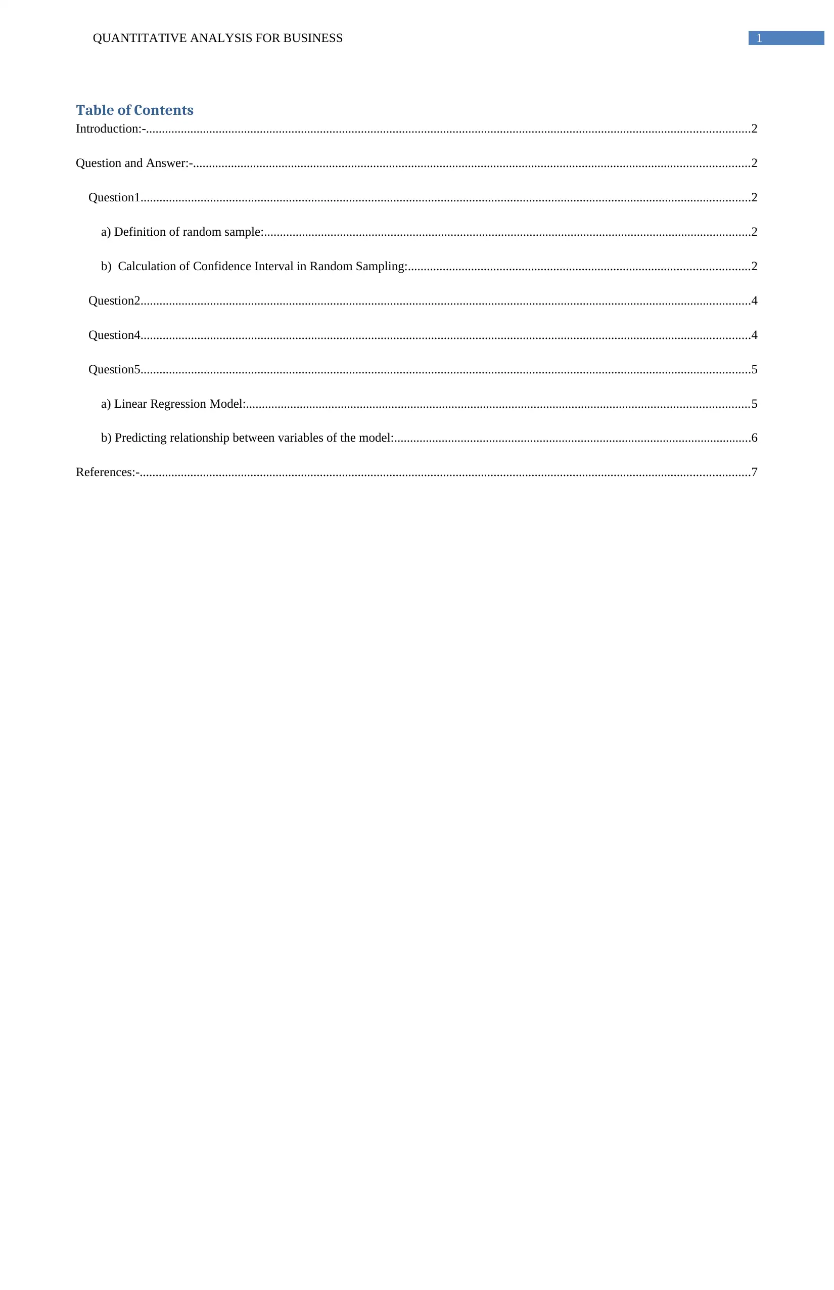
Table of Contents
Introduction:-...............................................................................................................................................................................................2
Question and Answer:-................................................................................................................................................................................2
Question1.................................................................................................................................................................................................2
a) Definition of random sample:..........................................................................................................................................................2
b) Calculation of Confidence Interval in Random Sampling:............................................................................................................2
Question2.................................................................................................................................................................................................4
Question4.................................................................................................................................................................................................4
Question5.................................................................................................................................................................................................5
a) Linear Regression Model:...............................................................................................................................................................5
b) Predicting relationship between variables of the model:.................................................................................................................6
References:-.................................................................................................................................................................................................7

QUANTITATIVE ANALYSIS FOR BUSINESS 2
Introduction:-
The report includes the answers of 4 questions and their subparts. With the help of MS excel the calculation and analysis was
incorporated. The necessary tables and figures were given in the report for interpretation of the results and answers. The report does
not provide any screen shots as per instruction in the assignment. The help was taken from statistical analysis oriented materials and
articles to complete the assignment. We also have drawn inferences as applicable in the calculation.
Question and Answer:-
Question1.
a) Definition of random sample:
Random sample is simply a subset of individuals chosen from a larger set of population. Each sample is selected randomly. Each
sample has the same probability of being chosen with same probability at any phase during the sampling process.
For example, cards are drawn from a deck, it is important that the deck be thoroughly mixed. The random sampling method is
mainly of two types: one is SRSWR (simple random sampling with replacement) and other is SRSWOR (simple random sampling
without replacement) (Chaum 2017). The simple random sampling with replacement is the process of drawing random samples where
samples already drawn from a population are not replaced in the population. The simple random sampling without replacement is the
method of drawing where samples already drawn from a population are replaced in the population. Always sample size is smaller in
number with respect to population. Random sample drawing and analysis helps us to realize the whole population.
b) Calculation of Confidence Interval in Random Sampling:
Quantra Ltd. (national wholesaler) delivers a range of branded products to retailers with a recommended retail price for each
product. In a random sample out of 200 retailers, it was found that 79 retailers sold products below price.
We can assert a null hypothesis against alternative hypothesis-
Null hypothesis (H0) = proportion of retailers that are selling products below the selling price is significant.
Alternative Hypothesis (HA) = proportion of retailers that are selling products below the selling price is insignificant.
Solution:
For large number of random samples a confidence interval for a population proportion is given by –
sample proportion +/- z*square root [(sample proportion*(1 – sample proportion)/total number of the sample].
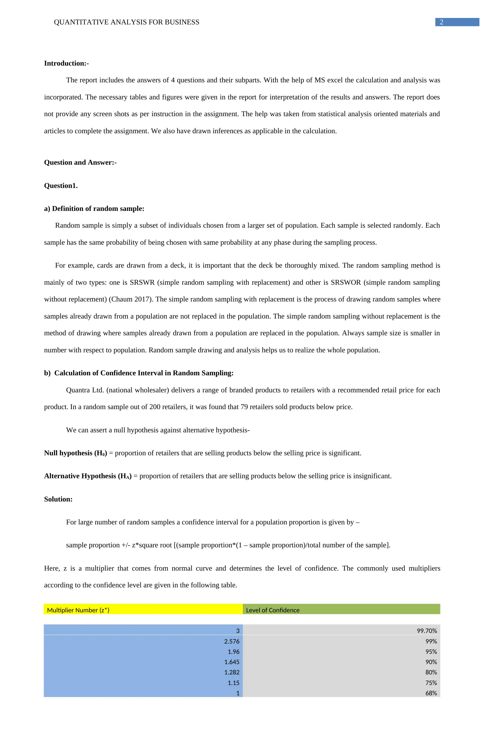
Here, z is a multiplier that comes from normal curve and determines the level of confidence. The commonly used multipliers
according to the confidence level are given in the following table.
Multiplier Number (z*) Level of Confidence
3 99.70%
2.576 99%
1.96 95%
1.645 90%
1.282 80%
1.15 75%
1 68%

QUANTITATIVE ANALYSIS FOR BUSINESS 3
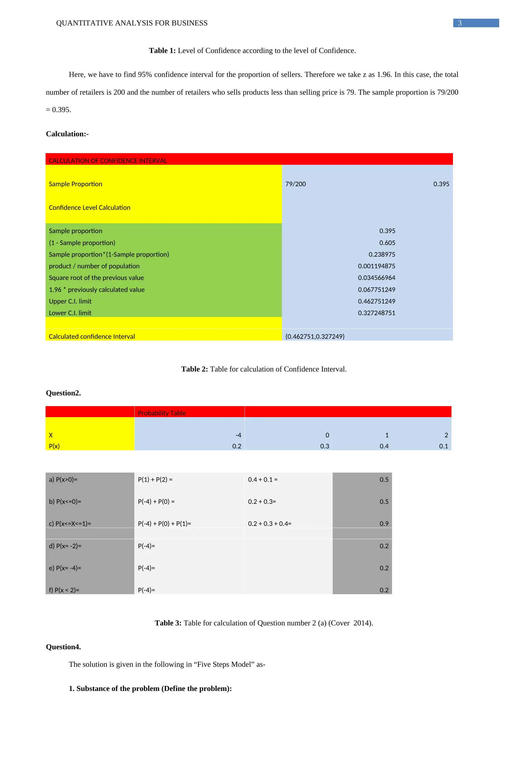
Table 1: Level of Confidence according to the level of Confidence.
Here, we have to find 95% confidence interval for the proportion of sellers. Therefore we take z as 1.96. In this case, the total
number of retailers is 200 and the number of retailers who sells products less than selling price is 79. The sample proportion is 79/200
= 0.395.
Calculation:-
CALCULATION OF CONFIDENCE INTERVAL
Sample Proportion 79/200 0.395
Confidence Level Calculation
Sample proportion 0.395
(1 - Sample proportion) 0.605
Sample proportion*(1-Sample proportion) 0.238975
product / number of population 0.001194875
Square root of the previous value 0.034566964
1.96 * previously calculated value 0.067751249
Upper C.I. limit 0.462751249
Lower C.I. limit 0.327248751
Calculated confidence Interval (0.462751,0.327249)
Table 2: Table for calculation of Confidence Interval.
Question2.
Probability Table
X -4 0 1 2
P(x) 0.2 0.3 0.4 0.1
a) P(x>0)= P(1) + P(2) = 0.4 + 0.1 = 0.5
b) P(x<=0)= P(-4) + P(0) = 0.2 + 0.3= 0.5
c) P(x<=X<=1)= P(-4) + P(0) + P(1)= 0.2 + 0.3 + 0.4= 0.9
d) P(x= -2)= P(-4)= 0.2
e) P(x= -4)= P(-4)= 0.2
f) P(x < 2)= P(-4)= 0.2
Table 3: Table for calculation of Question number 2 (a) (Cover 2014).
Question4.
The solution is given in the following in “Five Steps Model” as-
1. Substance of the problem (Define the problem):

QUANTITATIVE ANALYSIS FOR BUSINESS 4
Homes in Blacktown city have a mean value of $88950. It is assumed that homes in vicinity of the city have a higher value. To
test the hypothesis, a random sample of 12 homes is selected from the city area. The mean valuation of 12 homes is $92460 and
standard deviation is $5200. We assume that the prices of the homes are normally distributed.
2. Hypothesis Testing (Determination of testing objectives):
Now, we make a hypothesis leveling population standard deviation as Sigma1 square and sample standard deviation as Sigma2
square at alpha = 0.05, that-
Null hypothesis (H0): The standard deviation of total population and random samples are equal. (Sigma1 square = Sigma2
square, that is (Sigma1 square - Sigma2 square) = 0).
Alternative hypothesis (HA): The standard deviation of total population and random samples are unequal. (Sigma1 square =/
Sigma2 square, that is (Sigma1 square - Sigma2 square) =/ 0).
3. Feedback and assessment learning:
Here, let us assume the number of homes in the home time city is greater than 30 (N>30). 12 random samples are taken from
that population. Therefore, X-bar = $88950, x-bar = $92460. Sigma1 = unknown, Sigma2 = $5200, n = the number of random samples
= 12. We have n = 12. Degrees of freedom (df) = 12 -1 =11. We have the critical region (alpha) = 0.05. Hence the critical region is 5%
and we have to find (100-5) %=95% confidence interval.
4. Pick one solution from the brainstorming solutions:
Different types of tests such as t-test, z-test, chi-square test, F-test are available for finding out the confidence interval.
However, here standard deviation of sample is known along with the known means of population and sample. Based on the sample
size and sample standard deviation (Sigma1 square, we are trying to calculate confidence interval of population standard deviation
(Sigma2 square). Therefore chi-square test would be the exact test to implement for testing the assigned hypothesis (Schumacker and
Tomek 2013).
5. Implementation of solving strategy (Finding out the result):
A 95% confidence interval gives 2.5% of the area at each end of a chi-square distribution (Sengers and Anisimov 2016). We
found the values chi-square (df=0.975) = 13.8444 and chi-square (df=0.025) = 41.923 from the chi-distribution table.
Evaluating, [(n-1)*Sigma22/chi-square value], we obtain the values 1364.41 <= Sigma12<= 4131.75 (Farnsworth 2016).
The 95% confidence interval of standard deviation of Blacktown city is found to be (1364.41, 4131.75). This interval does not
contain Sigma2 square value ($5200). For a small amount of critical region (0.05), standard deviation of the population has 95%
probability to be unequal to Sigma2 square value. Therefore, we reject the null hypothesis and accept the alternative hypothesis of
unequal standard deviation.
Question5.
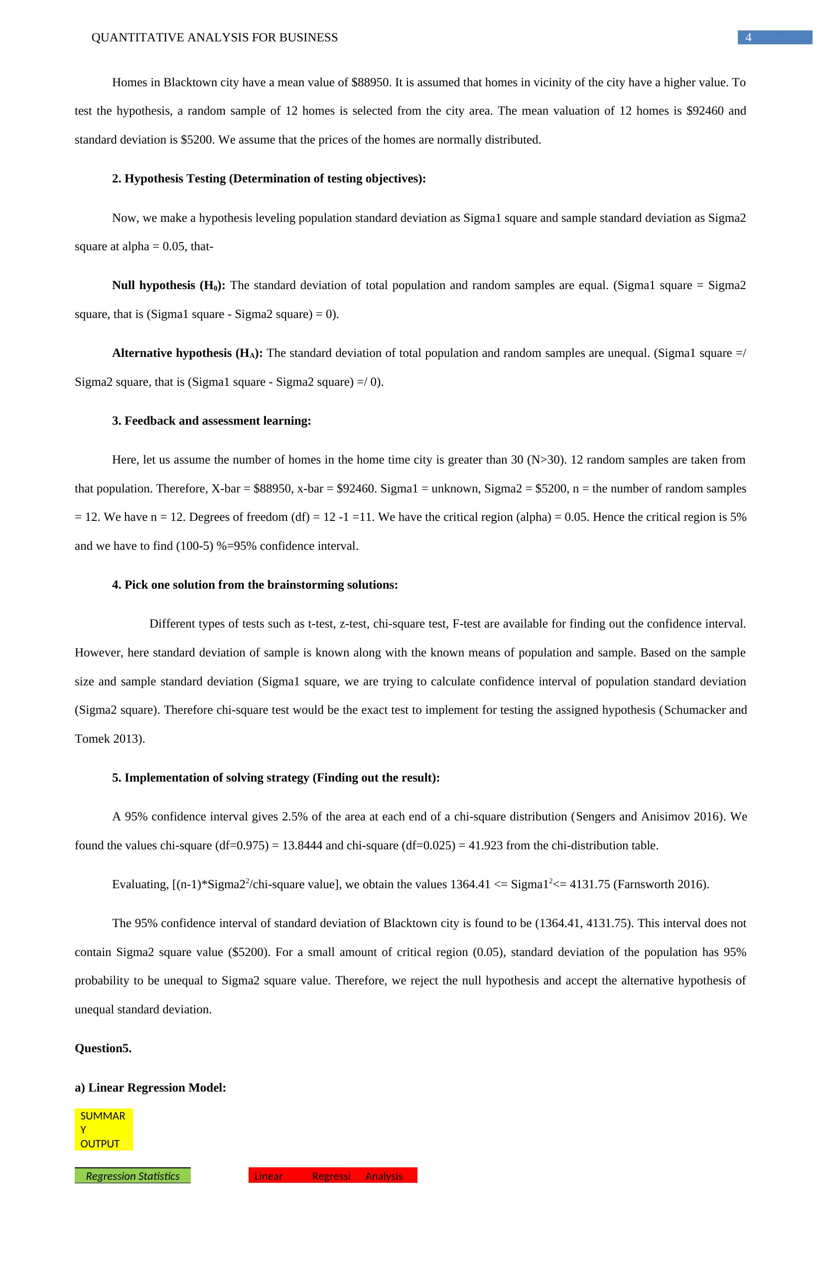
a) Linear Regression Model:
SUMMAR
Y
OUTPUT
Regression Statistics Linear Regressi Analysis

QUANTITATIVE ANALYSIS FOR BUSINESS 5
on
Multiple
R
0.994194
942
R Square
0.988423
583
Units of
Outputs vs. Cost
Adjusted
R Square
0.986494
18
Standard
Error
1.583737
252
Observati
ons 8
ANOVA
df SS MS F
Significan
ce F
Regressio
n 1
1284.950
658
1284.950
658
512.295
082
4.8693E-
07
Residual 6
15.04934
211
2.508223
684
Total 7 1300
Coefficien
ts
Standard
Error t Stat P-value
Lower
95%
Upper
95%
Lower
95.0%
Upper
95.0%
Intercept
-
21.46792
763
2.449244
904
-
8.765120
873
0.00012
217
-
27.46101
4
-
15.47484
13
-
27.46101
4
-
15.47484
126
Cost
1.027960
526
0.045416
78
22.63393
651
4.8693E-
07
0.916829
668
1.139091
385
0.916829
668
1.139091
385
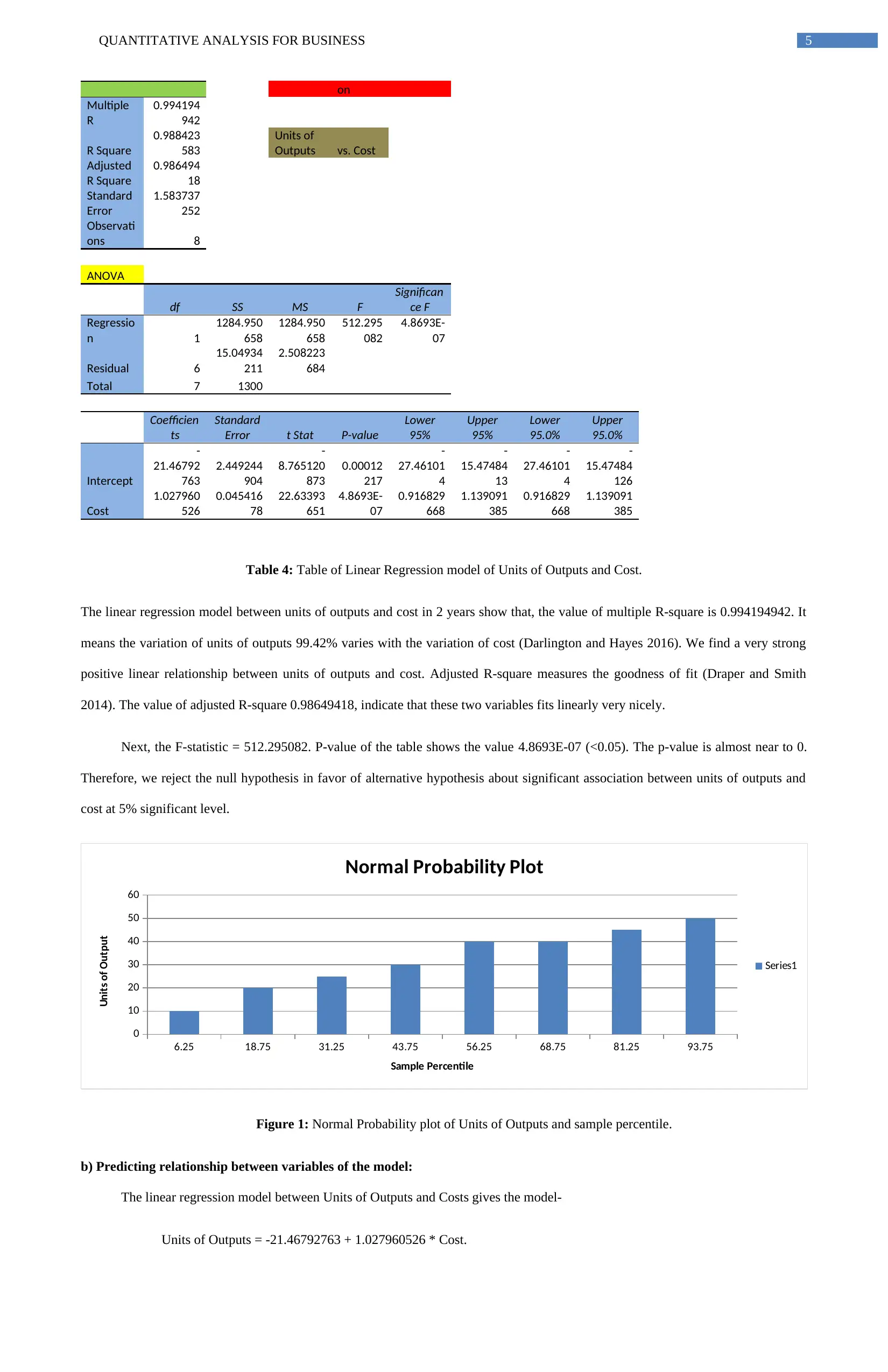
Table 4: Table of Linear Regression model of Units of Outputs and Cost.
The linear regression model between units of outputs and cost in 2 years show that, the value of multiple R-square is 0.994194942. It
means the variation of units of outputs 99.42% varies with the variation of cost (Darlington and Hayes 2016). We find a very strong
positive linear relationship between units of outputs and cost. Adjusted R-square measures the goodness of fit (Draper and Smith
2014). The value of adjusted R-square 0.98649418, indicate that these two variables fits linearly very nicely.
Next, the F-statistic = 512.295082. P-value of the table shows the value 4.8693E-07 (<0.05). The p-value is almost near to 0.
Therefore, we reject the null hypothesis in favor of alternative hypothesis about significant association between units of outputs and
cost at 5% significant level.
6.25 18.75 31.25 43.75 56.25 68.75 81.25 93.75
0
10
20
30
40
50
60
Normal Probability Plot
Series1
Sample Percentile
Units of Output
Figure 1: Normal Probability plot of Units of Outputs and sample percentile.
b) Predicting relationship between variables of the model:
The linear regression model between Units of Outputs and Costs gives the model-
Units of Outputs = -21.46792763 + 1.027960526 * Cost.

QUANTITATIVE ANALYSIS FOR BUSINESS 6
The value of R-square and adjusted R-square interprets that these two values are highly linearly related. However, the value of
Significance of F-statistic indicates that they do not have strong association between themselves.
Units of Outputs Cost
Units of Outputs 1 0.994194942
Cost 0.994194942 1
Table 5: Correlation coefficient between Units of Outputs and Cost.
The Person’s correlation coefficient between Units of Outputs and Cost is 0.994194942. Therefore, we can interpret that these
two variables are highly correlated with each other (Ye 2013).

QUANTITATIVE ANALYSIS FOR BUSINESS 7
References:-
Chaum, D., 2017. Random sample elections. U.S. Patent Application 15/405,395.
Cover, T.M., 2014. A hierarchy of probability density function estimates. Frontiers in Pattern Recognition, pp.83-98.
Darlington, R.B. and Hayes, A.F., 2016. Regression analysis and linear models: Concepts, applications, and implementation. Guilford
Publications.
Draper, N.R. and Smith, H., 2014. Applied regression analysis. John Wiley & Sons.
Farnsworth, D.L., 2016. CONFIDENCE INTERVALS INSTEAD OF HYPOTHESIS TESTS. Mathematics and Computer Education,
50(2), p.130.
Schumacker, R. and Tomek, S., 2013. Chi-square test. In Understanding Statistics Using R (pp. 169-175). Springer New York.
Sengers, J.V. and Anisimov, M.A., 2016. Critical Region. International Union of Pure and Applied Chemistry.
Ye, J., 2013. Multicriteria decision-making method using the correlation coefficient under single-valued neutrosophic environment.
International Journal of General Systems, 42(4), pp.386-394.