Quantitative Methods for Accounting & Finance

The text discusses various topics related to quantitative methods for accounting & finance such as hypothesis testing, confidence intervals, regression analysis and more. It provides solutions to problems and explains concepts in detail. Desklib is an online library that provides solved assignments, essays, dissertations and study material for students.

Quantitative Methods for Accounting & Finance

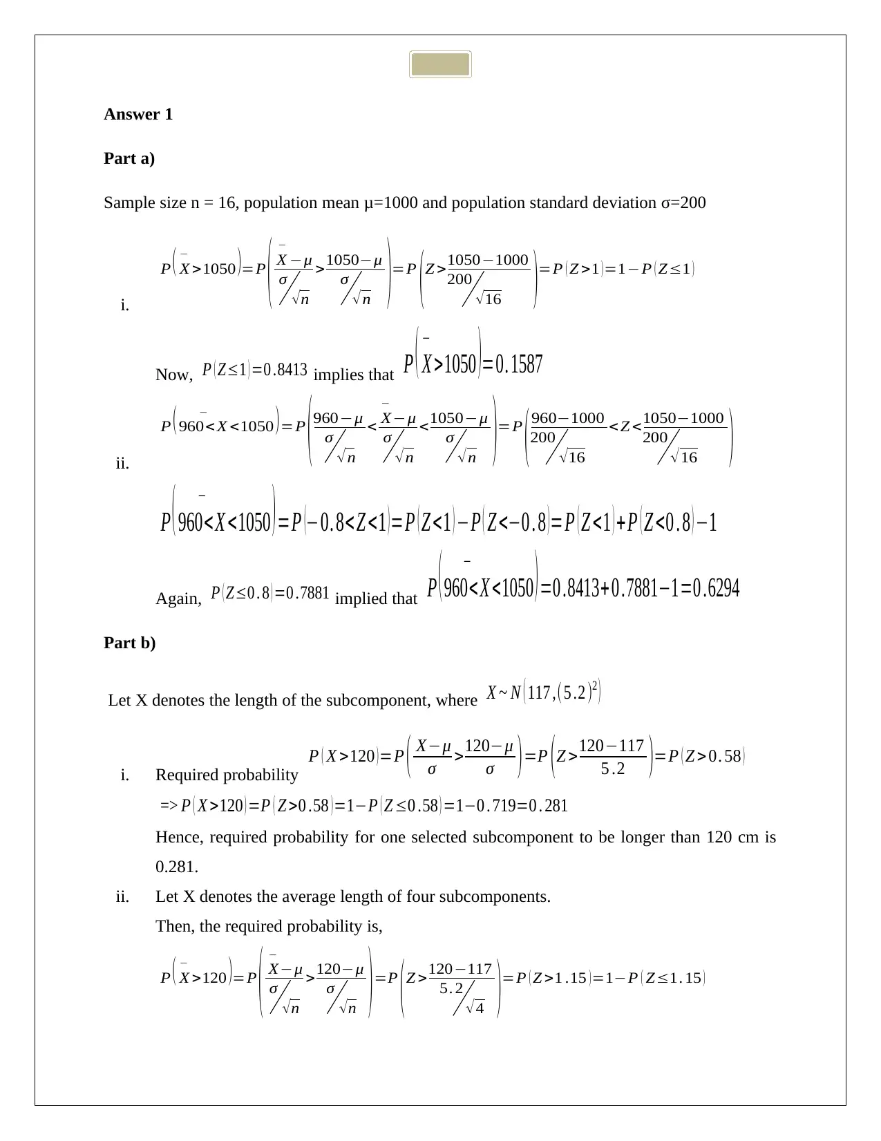
Answer 1
Part a)
Sample size n = 16, population mean μ=1000 and population standard deviation σ=200
i.
P ( X
−
>1050 )=P
( X
−
−μ
σ
√ n
>1050−μ
σ
√ n )=P
( Z >1050−1000
200
√ 16 )=P ( Z >1 ) =1−P ( Z≤1 )
Now, P ( Z≤1 ) =0 .8413 implies that P ( X
−
>1050 )=0. 1587
ii.
P ( 960< X
−
<1050 ) =P
( 960−μ
σ
√ n
< X
−
−μ
σ
√ n
<1050−μ
σ
√ n )=P
( 960−1000
200
√ 16
< Z <1050−1000
200
√ 16 )
P ( 960<X
−
<1050 ) =P (−0. 8< Z <1 ) =P ( Z <1 ) −P ( Z <−0 . 8 ) =P ( Z <1 ) +P ( Z <0 . 8 ) −1
Again, P ( Z≤0 . 8 ) =0 .7881 implied that P ( 960< X
−
<1050 ) =0 .8413+ 0 .7881−1=0 .6294
Part b)
Let X denotes the length of the subcomponent, where X ~ N ( 117 ,(5 .2 )2 )
i. Required probability
P ( X >120 ) =P ( X−μ
σ >120−μ
σ ) =P ( Z >120−117
5 .2 )=P ( Z > 0. 58 )
=> P ( X >120 ) =P ( Z >0 .58 ) =1−P ( Z ≤0 .58 ) =1−0 . 719=0 . 281
Hence, required probability for one selected subcomponent to be longer than 120 cm is
0.281.
ii. Let X denotes the average length of four subcomponents.
Then, the required probability is,
P ( X
−
>120 )=P
( X
−
−μ
σ
√ n
>120−μ
σ
√ n ) =P
( Z >120−117
5. 2
√ 4 )=P ( Z >1 .15 ) =1−P ( Z≤1. 15 )

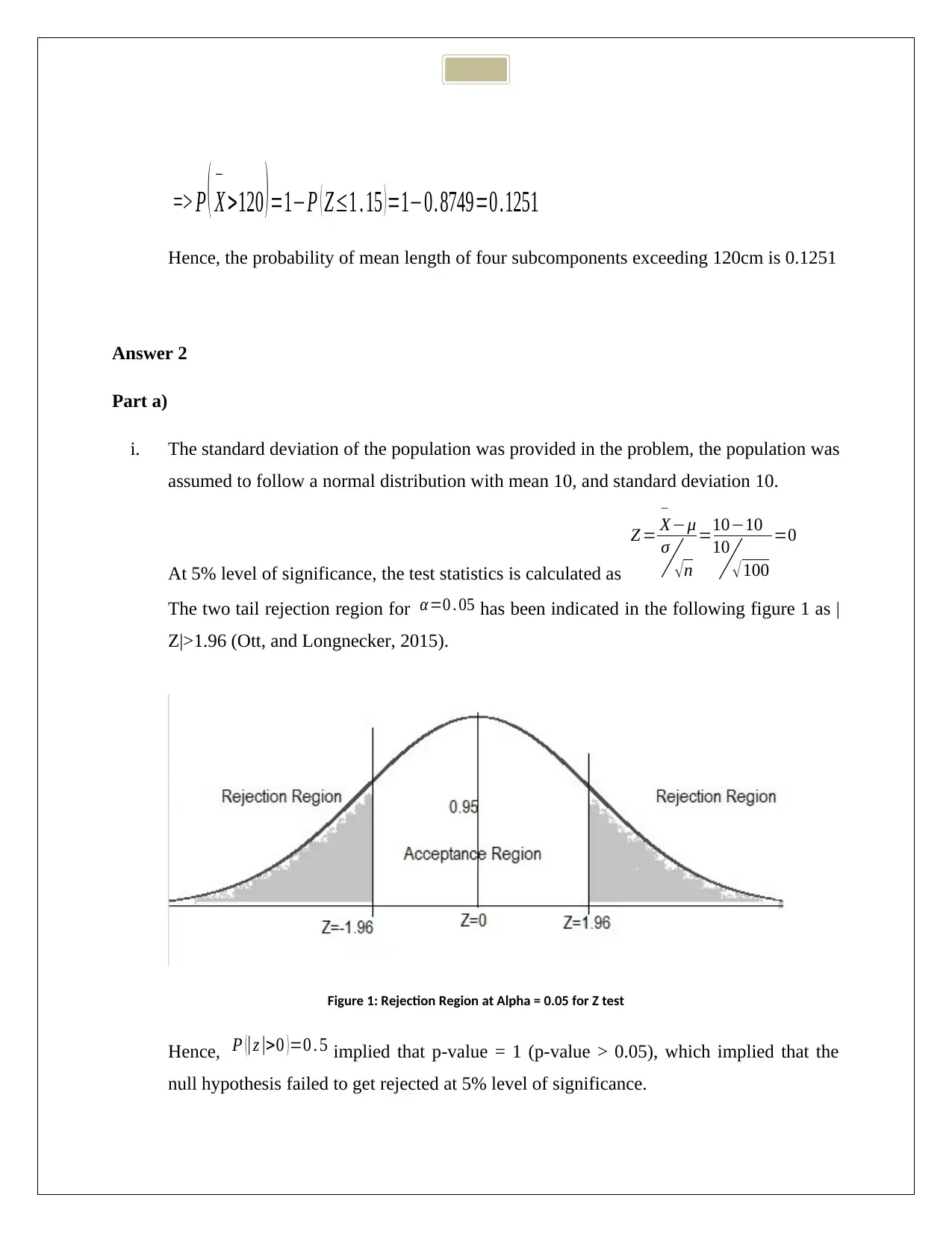
=> P ( X
−
>120 ) =1−P ( Z≤1 . 15 ) =1−0. 8749=0 .1251
Hence, the probability of mean length of four subcomponents exceeding 120cm is 0.1251
Answer 2
Part a)
i. The standard deviation of the population was provided in the problem, the population was
assumed to follow a normal distribution with mean 10, and standard deviation 10.
At 5% level of significance, the test statistics is calculated as
Z = X
−
−μ
σ
√ n
=10−10
10
√ 100
=0
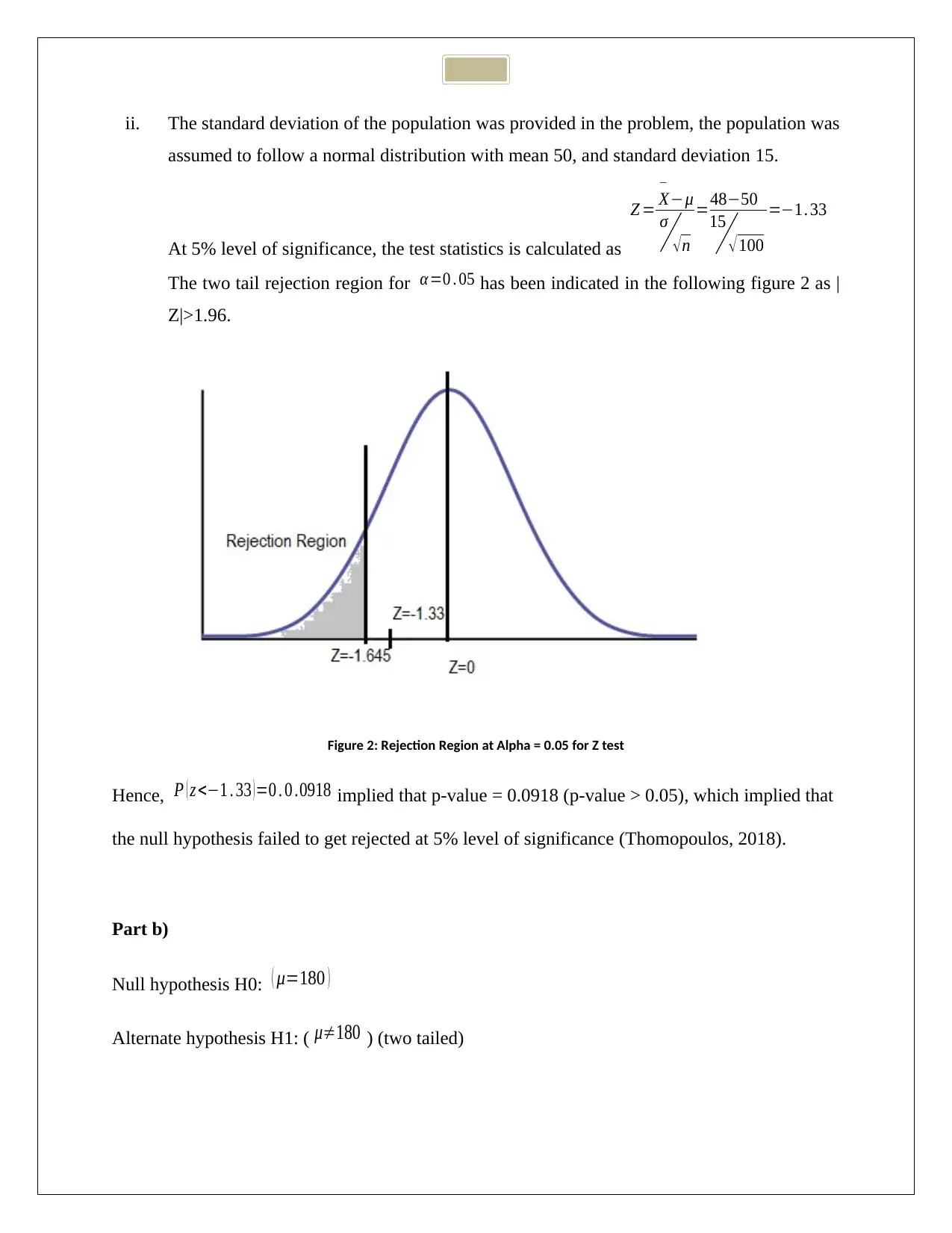
The two tail rejection region for α =0 . 05 has been indicated in the following figure 1 as |
Z|>1.96 (Ott, and Longnecker, 2015).
Figure 1: Rejection Region at Alpha = 0.05 for Z test
Hence, P (|z|>0 ) =0 . 5 implied that p-value = 1 (p-value > 0.05), which implied that the
null hypothesis failed to get rejected at 5% level of significance.

ii. The standard deviation of the population was provided in the problem, the population was
assumed to follow a normal distribution with mean 50, and standard deviation 15.
At 5% level of significance, the test statistics is calculated as
Z = X
−
−μ
σ
√ n
=48−50
15
√ 100
=−1. 33
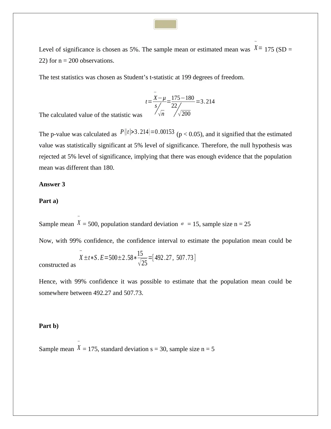
The two tail rejection region for α =0 . 05 has been indicated in the following figure 2 as |
Z|>1.96.
Figure 2: Rejection Region at Alpha = 0.05 for Z test
Hence, P ( z <−1 . 33 ) =0 . 0 .0918 implied that p-value = 0.0918 (p-value > 0.05), which implied that
the null hypothesis failed to get rejected at 5% level of significance (Thomopoulos, 2018).
Part b)
Null hypothesis H0: ( μ=180 )
Alternate hypothesis H1: ( μ≠180 ) (two tailed)

Level of significance is chosen as 5%. The sample mean or estimated mean was X
−
= 175 (SD =
22) for n = 200 observations.
The test statistics was chosen as Student’s t-statistic at 199 degrees of freedom.
The calculated value of the statistic was
t= X
−
−μ
s
√ n
=175−180
22
√ 200
=3. 214
The p-value was calculated as P (|t|>3 . 214 ) =0 .00153 (p < 0.05), and it signified that the estimated
value was statistically significant at 5% level of significance. Therefore, the null hypothesis was
rejected at 5% level of significance, implying that there was enough evidence that the population
mean was different than 180.
Answer 3
Part a)
Sample mean X
−
= 500, population standard deviation σ = 15, sample size n = 25
Now, with 99% confidence, the confidence interval to estimate the population mean could be
constructed as
X
−
±t∗S . E=500±2 .58∗15
√ 25 =[ 492 .27 , 507 .73 ]
Hence, with 99% confidence it was possible to estimate that the population mean could be
somewhere between 492.27 and 507.73.
Part b)
Sample mean X
−
= 175, standard deviation s = 30, sample size n = 5

Now, with 90% confidence, the confidence interval to estimate the population mean could be
constructed as
X
−
±t∗S . E=175±2 .13∗30
√ 5 =[ 146. 4 , 203 . 6 ]
Hence, with 90% confidence it was possible to estimate that the population mean could be
somewhere between 146.4 and 203.6 (Hopkins, 2017)
Answer 4
To test the difference of two population averages, Z-test was used as follows (Chatfield, 2018).
Null hypothesis H0: ( μ1−μ2 = 0)
Alternate hypothesis HA: ( μ1−μ2<¿ ¿ 0) (left tail test)
Level of significance for the test was chosen as 10%, that is α =0 . 1
Sample data available for sample 1 were X1
−
=51. 3 , σ12=52, n1=31 and for sample 2 were
X2
−
=53 .2 , σ 22=60 , n2=32
The test statistic was calculated as
Z = ( X
−
1−X
−
2 ) −d
SE where SE was calculated as
SE= √ σ1
2
n1
+ σ 2
2
n 2= √ 52
31 +60
32 =1 . 885 , d=μ1−μ2=0 . So, Z =51. 3−53 . 2
1. 885 =−1 . 008
The p-value was calculated as P ( Z <−1 .008 ) =0 .1567
The critical value of the test statistic was calculated as Z = -1.2816

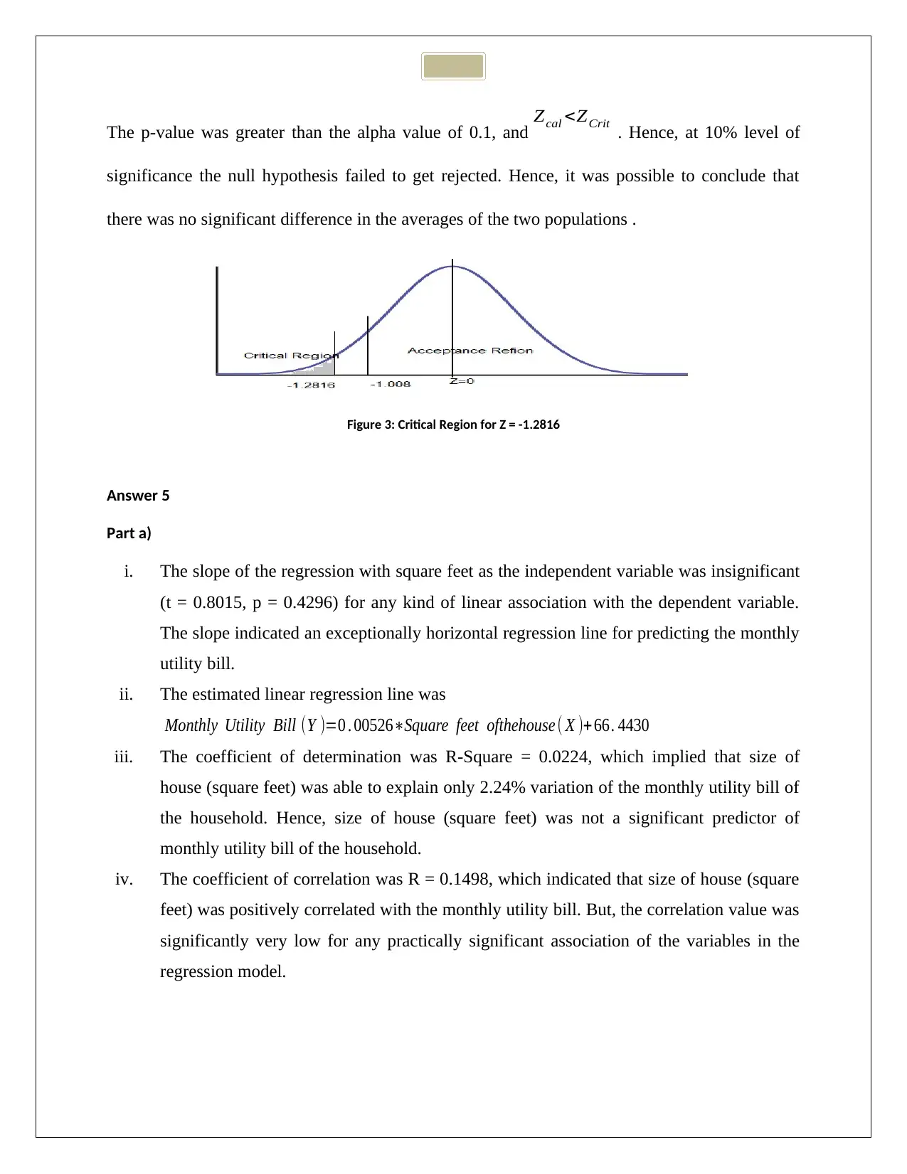
The p-value was greater than the alpha value of 0.1, and Zcal <ZCrit . Hence, at 10% level of
significance the null hypothesis failed to get rejected. Hence, it was possible to conclude that
there was no significant difference in the averages of the two populations .
Figure 3: Critical Region for Z = -1.2816
Answer 5
Part a)
i. The slope of the regression with square feet as the independent variable was insignificant
(t = 0.8015, p = 0.4296) for any kind of linear association with the dependent variable.
The slope indicated an exceptionally horizontal regression line for predicting the monthly
utility bill.
ii. The estimated linear regression line was
Monthly Utility Bill (Y )=0 . 00526∗Square feet ofthehouse ( X )+ 66. 4430
iii. The coefficient of determination was R-Square = 0.0224, which implied that size of
house (square feet) was able to explain only 2.24% variation of the monthly utility bill of
the household. Hence, size of house (square feet) was not a significant predictor of
monthly utility bill of the household.
iv. The coefficient of correlation was R = 0.1498, which indicated that size of house (square
feet) was positively correlated with the monthly utility bill. But, the correlation value was
significantly very low for any practically significant association of the variables in the
regression model.

Part b)
In the southern state, size of houses was assumed to be a significant predictor of the
monthly utility bills of the house. But, on the contrary, no significant relation between the
two variables was found. Size of the house was able to explain mere 2.24% variation in
the monthly utility bills. The regression model indicated that for increase in one square
unit of house, monthly utility bills would go up by a factor of 0.0053. The intercept of
66.443 indicated that monthly utility bill would be $ 66.44, even for zero size of the
house (square feet). Practically, the model indicated existence of other significant
independent impact factors affecting the monthly utility bills.
References
Chatfield, C., 2018. Statistics for technology: a course in applied statistics. Routledge.
Hopkins, W.G., 2017. A Spreadsheet for Deriving a Confidence Interval, Mechanistic Inference
and Clinical Inference from a P Value. Sportscience, 21.
Ott, R.L. and Longnecker, M.T., 2015. An introduction to statistical methods and data analysis.
Nelson Education.
Thomopoulos, N.T., 2018. Standard Normal. In Probability Distributions (pp. 45-55). Springer,
Cham.