Linear Regression Analysis of Expenditure Data

The assignment involves analyzing expenditure data using linear regression techniques. The student is required to calculate the Pearson correlation coefficient between age and expenditure, determine the significance of the relationship at a 1% level of significance, and perform a least square method for a log-linear model. The analysis reveals that expenditure has a moderate significant effect on age, but a better relationship is observed in the log-linear model compared to simple regression.

Running head: ADVANCED QUANTITATIVE METHODS FOR MANAGERS
Advanced Quantitative Methods for Managers
Name of the Student:
Name of the University:
Author’s note:

1ADVANCED QUANTITATIVE METHODS FOR MANAGERS
Table of Contents
Subject 1.....................................................................................................................................3
1.1. Hypotheses:.................................................................................................................3
1.2. Linear Regression Model:...........................................................................................3
1.3. Conclusion:..................................................................................................................3
1.4. Recommendation:........................................................................................................4
Subject 2.....................................................................................................................................4
2.1. Hypotheses:.....................................................................................................................4
2.2. Linear Regression Model:...............................................................................................4
2.3. Conclusion:.....................................................................................................................5
2.4. Recommendation:...........................................................................................................5
Subject 3.....................................................................................................................................5
3.1. Regression coefficients:..................................................................................................5
3.2. Linear Regression Equation:...........................................................................................6
3.3. Scatter Diagram:..............................................................................................................6
3.4. Slope, Intercept, Coefficient of Determination and F-statistic:......................................6
3.5. Correlation coefficient:...................................................................................................7
3.6. Significance at 1% level of significance:........................................................................7
Subject 4.....................................................................................................................................7
4.1. Linear Regression coefficients:.......................................................................................8
4.2. Linear Regression Equation:...........................................................................................8

2ADVANCED QUANTITATIVE METHODS FOR MANAGERS
4.3. Interpretation of b1:.........................................................................................................8
4.4. Scatter plot:.....................................................................................................................8
4.5. Difference between Linear Model and Log-Linear Model:............................................9
Conclusion:................................................................................................................................9
References:...............................................................................................................................10

3ADVANCED QUANTITATIVE METHODS FOR MANAGERS
Subject 1.
1.1. Hypotheses:
Null Hypothesis (H0): Knowledge does not have linear significant association with the
amount of Expenditures.
Alternative Hypothesis (HA): Knowledge have linear significant association with the amount
of Expenditures.
1.2. Linear Regression Model:
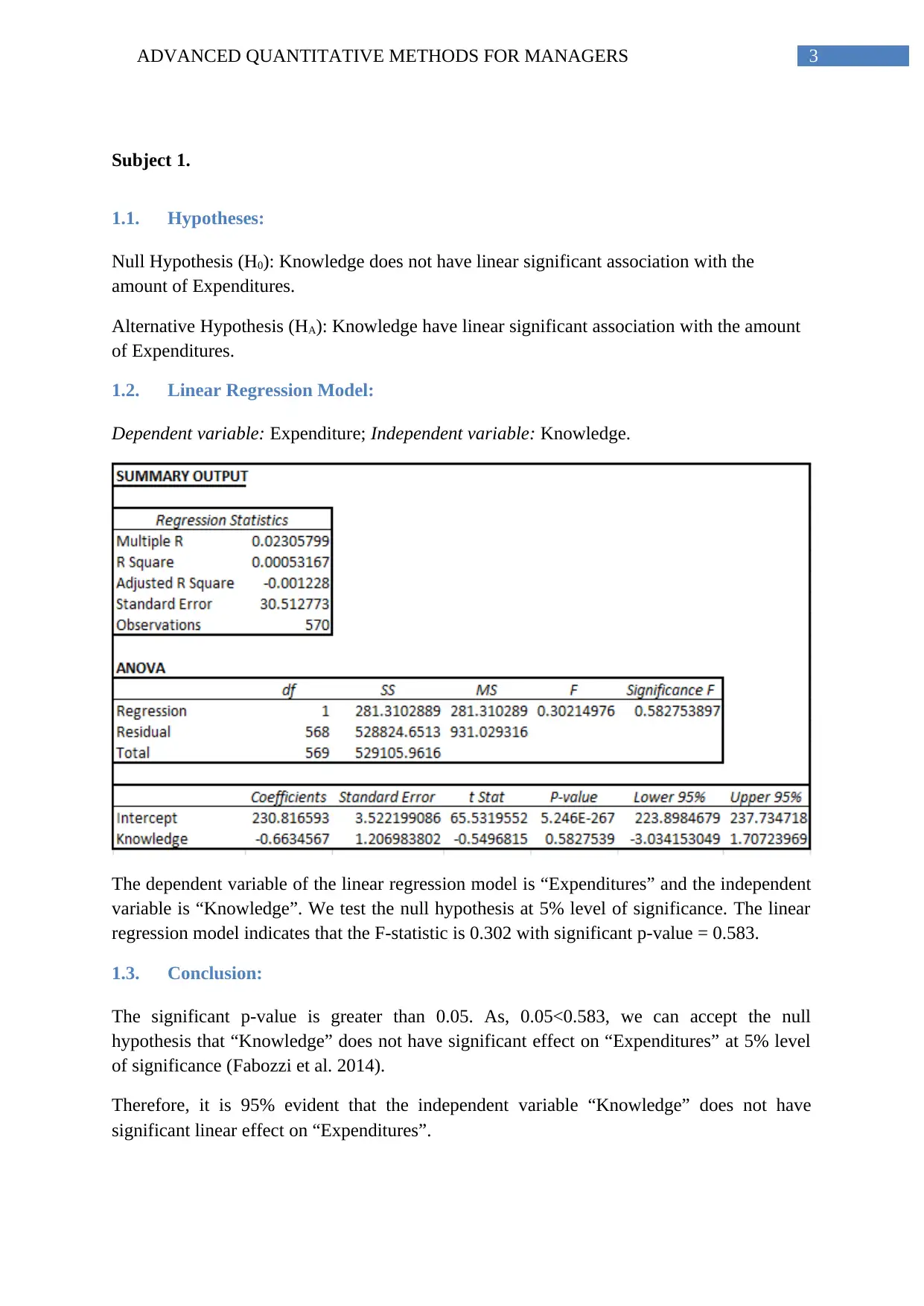
Dependent variable: Expenditure; Independent variable: Knowledge.
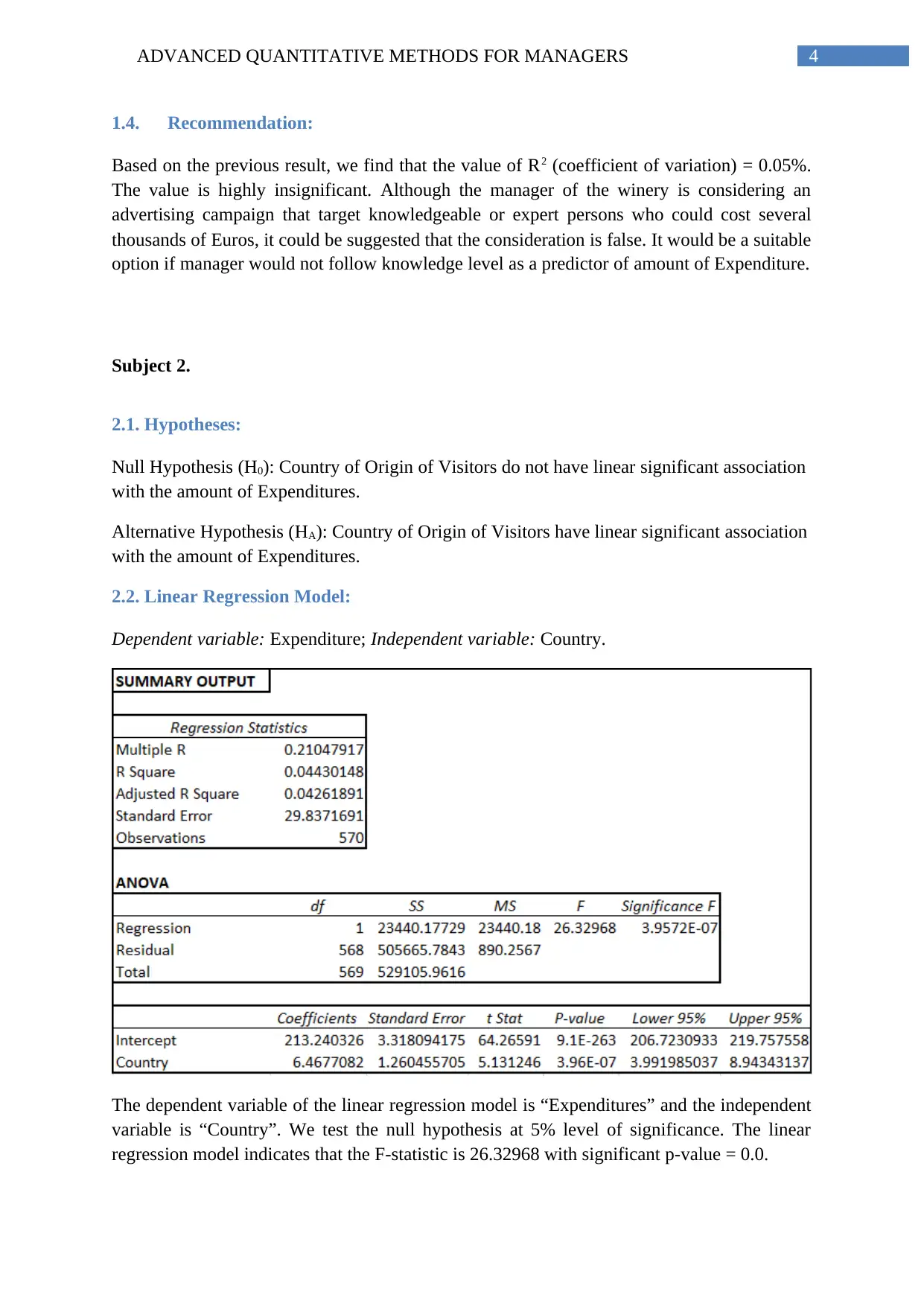
The dependent variable of the linear regression model is “Expenditures” and the independent
variable is “Knowledge”. We test the null hypothesis at 5% level of significance. The linear
regression model indicates that the F-statistic is 0.302 with significant p-value = 0.583.
1.3. Conclusion:
The significant p-value is greater than 0.05. As, 0.05<0.583, we can accept the null
hypothesis that “Knowledge” does not have significant effect on “Expenditures” at 5% level
of significance (Fabozzi et al. 2014).
Therefore, it is 95% evident that the independent variable “Knowledge” does not have
significant linear effect on “Expenditures”.

4ADVANCED QUANTITATIVE METHODS FOR MANAGERS
1.4. Recommendation:
Based on the previous result, we find that the value of R2 (coefficient of variation) = 0.05%.
The value is highly insignificant. Although the manager of the winery is considering an
advertising campaign that target knowledgeable or expert persons who could cost several
thousands of Euros, it could be suggested that the consideration is false. It would be a suitable
option if manager would not follow knowledge level as a predictor of amount of Expenditure.
Subject 2.
2.1. Hypotheses:
Null Hypothesis (H0): Country of Origin of Visitors do not have linear significant association
with the amount of Expenditures.
Alternative Hypothesis (HA): Country of Origin of Visitors have linear significant association
with the amount of Expenditures.
2.2. Linear Regression Model:
Dependent variable: Expenditure; Independent variable: Country.
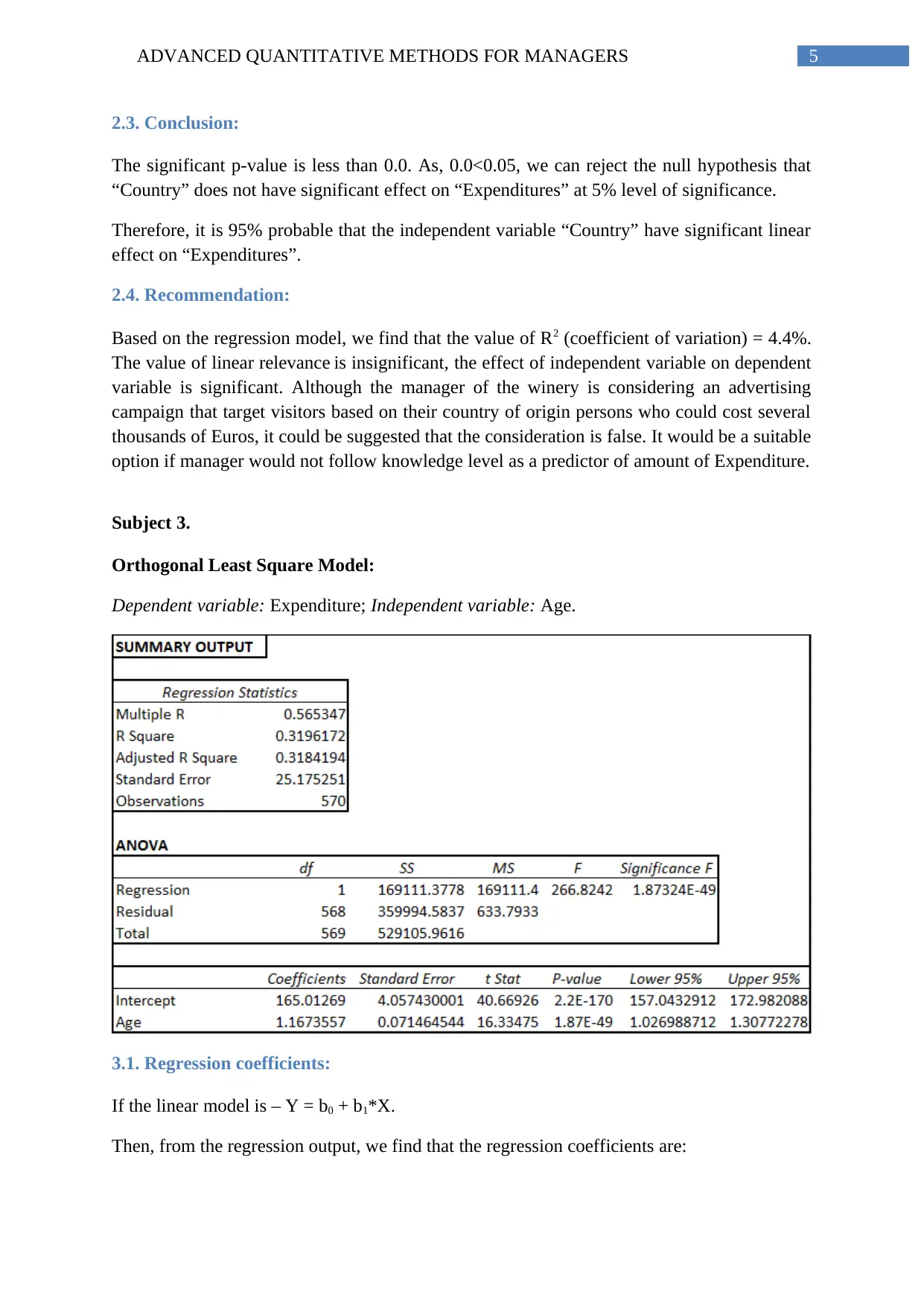
The dependent variable of the linear regression model is “Expenditures” and the independent
variable is “Country”. We test the null hypothesis at 5% level of significance. The linear
regression model indicates that the F-statistic is 26.32968 with significant p-value = 0.0.

5ADVANCED QUANTITATIVE METHODS FOR MANAGERS
2.3. Conclusion:
The significant p-value is less than 0.0. As, 0.0<0.05, we can reject the null hypothesis that
“Country” does not have significant effect on “Expenditures” at 5% level of significance.
Therefore, it is 95% probable that the independent variable “Country” have significant linear
effect on “Expenditures”.
2.4. Recommendation:
Based on the regression model, we find that the value of R2 (coefficient of variation) = 4.4%.
The value of linear relevance is insignificant, the effect of independent variable on dependent
variable is significant. Although the manager of the winery is considering an advertising
campaign that target visitors based on their country of origin persons who could cost several
thousands of Euros, it could be suggested that the consideration is false. It would be a suitable
option if manager would not follow knowledge level as a predictor of amount of Expenditure.
Subject 3.
Orthogonal Least Square Model:
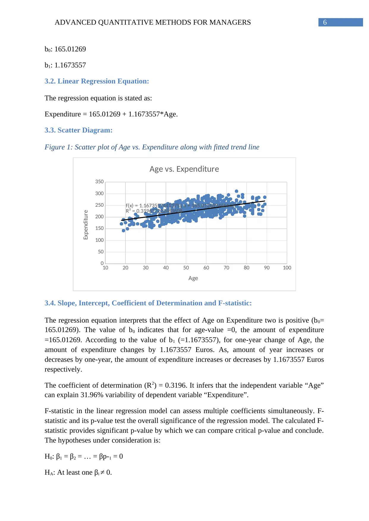
Dependent variable: Expenditure; Independent variable: Age.
3.1. Regression coefficients:
If the linear model is – Y = b0 + b1*X.
Then, from the regression output, we find that the regression coefficients are:

6ADVANCED QUANTITATIVE METHODS FOR MANAGERS
b0: 165.01269
b1: 1.1673557
3.2. Linear Regression Equation:
The regression equation is stated as:
Expenditure = 165.01269 + 1.1673557*Age.
3.3. Scatter Diagram:
Figure 1: Scatter plot of Age vs. Expenditure along with fitted trend line
10 20 30 40 50 60 70 80 90 100
0
50
100
150
200
250
300
350
f(x) = 1.16735574413751 x + 165.012689466145
R² = 0.319617222483608
Age vs. Expenditure
Age
Expenditure
3.4. Slope, Intercept, Coefficient of Determination and F-statistic:
The regression equation interprets that the effect of Age on Expenditure two is positive (b0=
165.01269). The value of b0 indicates that for age-value =0, the amount of expenditure
=165.01269. According to the value of b1 (=1.1673557), for one-year change of Age, the
amount of expenditure changes by 1.1673557 Euros. As, amount of year increases or
decreases by one-year, the amount of expenditure increases or decreases by 1.1673557 Euros
respectively.
The coefficient of determination (R2) = 0.3196. It infers that the independent variable “Age”
can explain 31.96% variability of dependent variable “Expenditure”.
F-statistic in the linear regression model can assess multiple coefficients simultaneously. F-
statistic and its p-value test the overall significance of the regression model. The calculated F-
statistic provides significant p-value by which we can compare critical p-value and conclude.
The hypotheses under consideration is:
H0: β1 = β2 = … = βp-1 = 0
HA: At least one βi ≠ 0.

7ADVANCED QUANTITATIVE METHODS FOR MANAGERS
3.5. Correlation coefficient:
The Pearson correlation co-efficient determines in which manner two variables are linked
with each other. The Pearson correlation coefficient is 0.565347. The correlation coefficient
depicts that Age and Expenditure are positively correlated. That is, if Age increases,
expenditure increases and if Age decreases, Expenditure decreases.
Besides, the correlation or link between Age and Expenditure is moderately strong (r = ±0.7
to ±0.3). Therefore, it is not strongly probable that for the increment or decrement of age, the
amount of expenditures also increases or decreases respectively.
3.6. Significance at 1% level of significance:
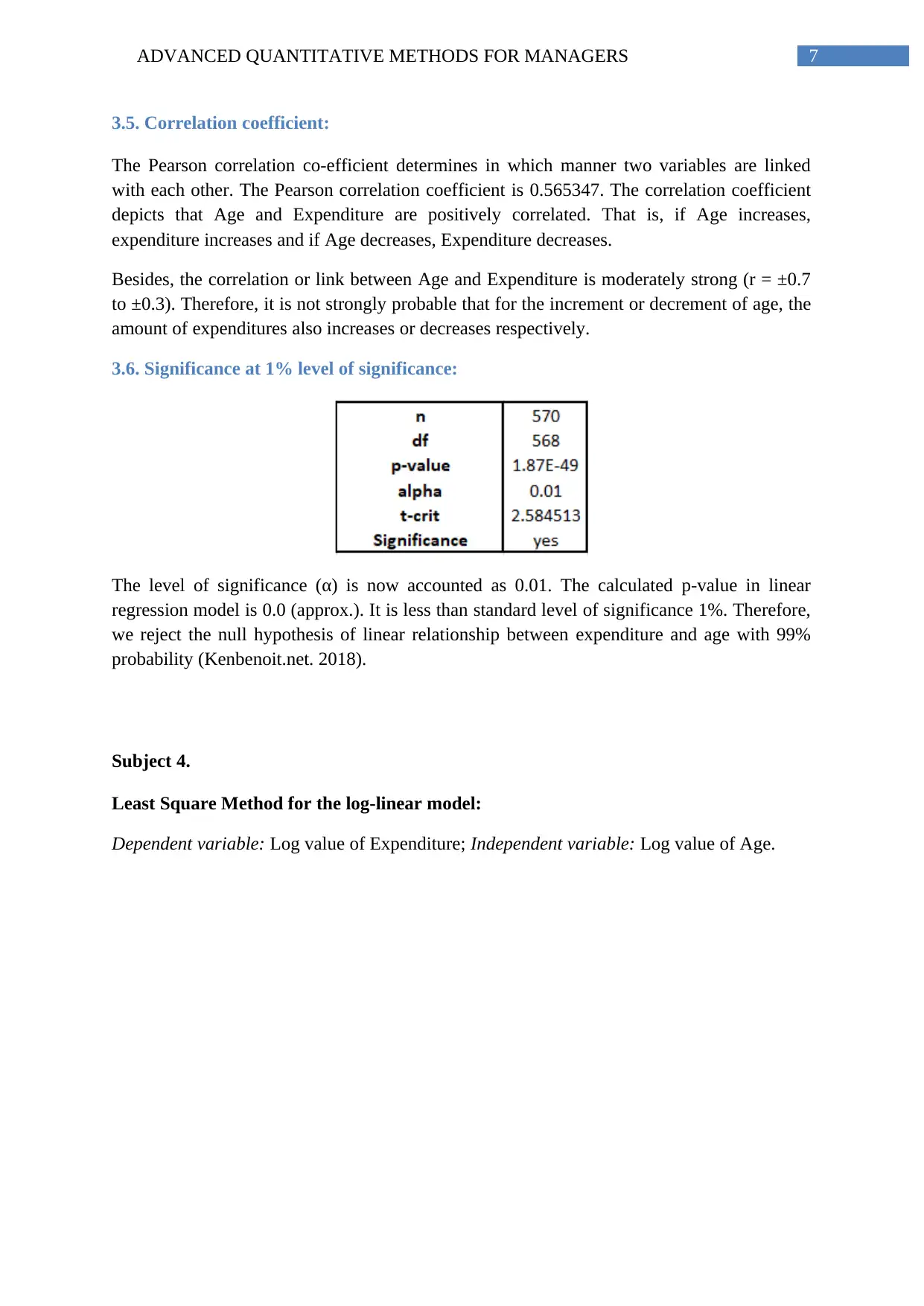
The level of significance (α) is now accounted as 0.01. The calculated p-value in linear
regression model is 0.0 (approx.). It is less than standard level of significance 1%. Therefore,
we reject the null hypothesis of linear relationship between expenditure and age with 99%
probability (Kenbenoit.net. 2018).
Subject 4.
Least Square Method for the log-linear model:
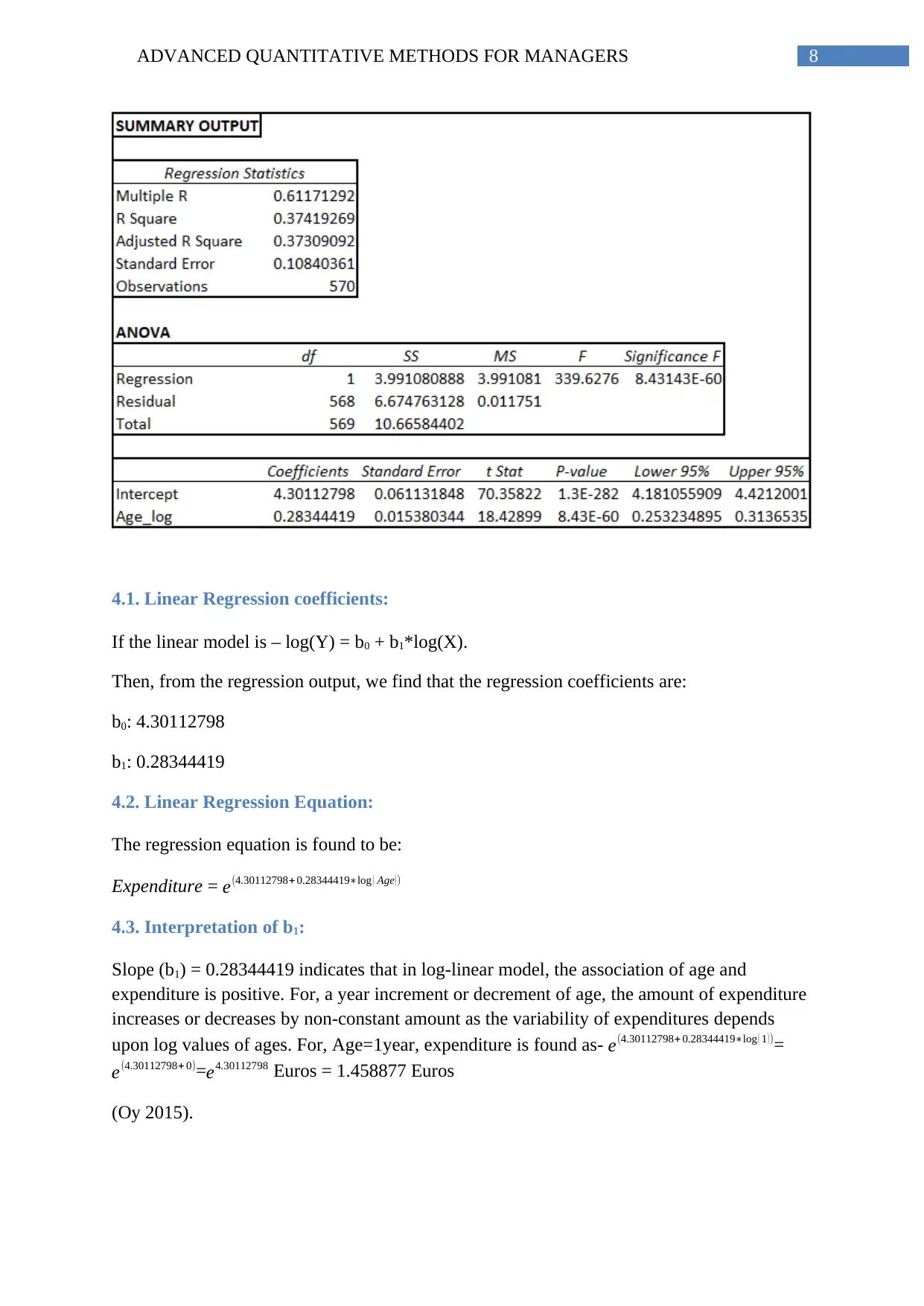
Dependent variable: Log value of Expenditure; Independent variable: Log value of Age.

8ADVANCED QUANTITATIVE METHODS FOR MANAGERS
4.1. Linear Regression coefficients:
If the linear model is – log(Y) = b0 + b1*log(X).
Then, from the regression output, we find that the regression coefficients are:
b0: 4.30112798
b1: 0.28344419
4.2. Linear Regression Equation:
The regression equation is found to be:
Expenditure = e(4.30112798+ 0.28344419∗log ( Age ))
4.3. Interpretation of b1:
Slope (b1) = 0.28344419 indicates that in log-linear model, the association of age and
expenditure is positive. For, a year increment or decrement of age, the amount of expenditure
increases or decreases by non-constant amount as the variability of expenditures depends
upon log values of ages. For, Age=1year, expenditure is found as- e(4.30112798+ 0.28344419∗log ( 1 ))=
e(4.30112798+ 0)=e4.30112798 Euros = 1.458877 Euros
(Oy 2015).

9ADVANCED QUANTITATIVE METHODS FOR MANAGERS
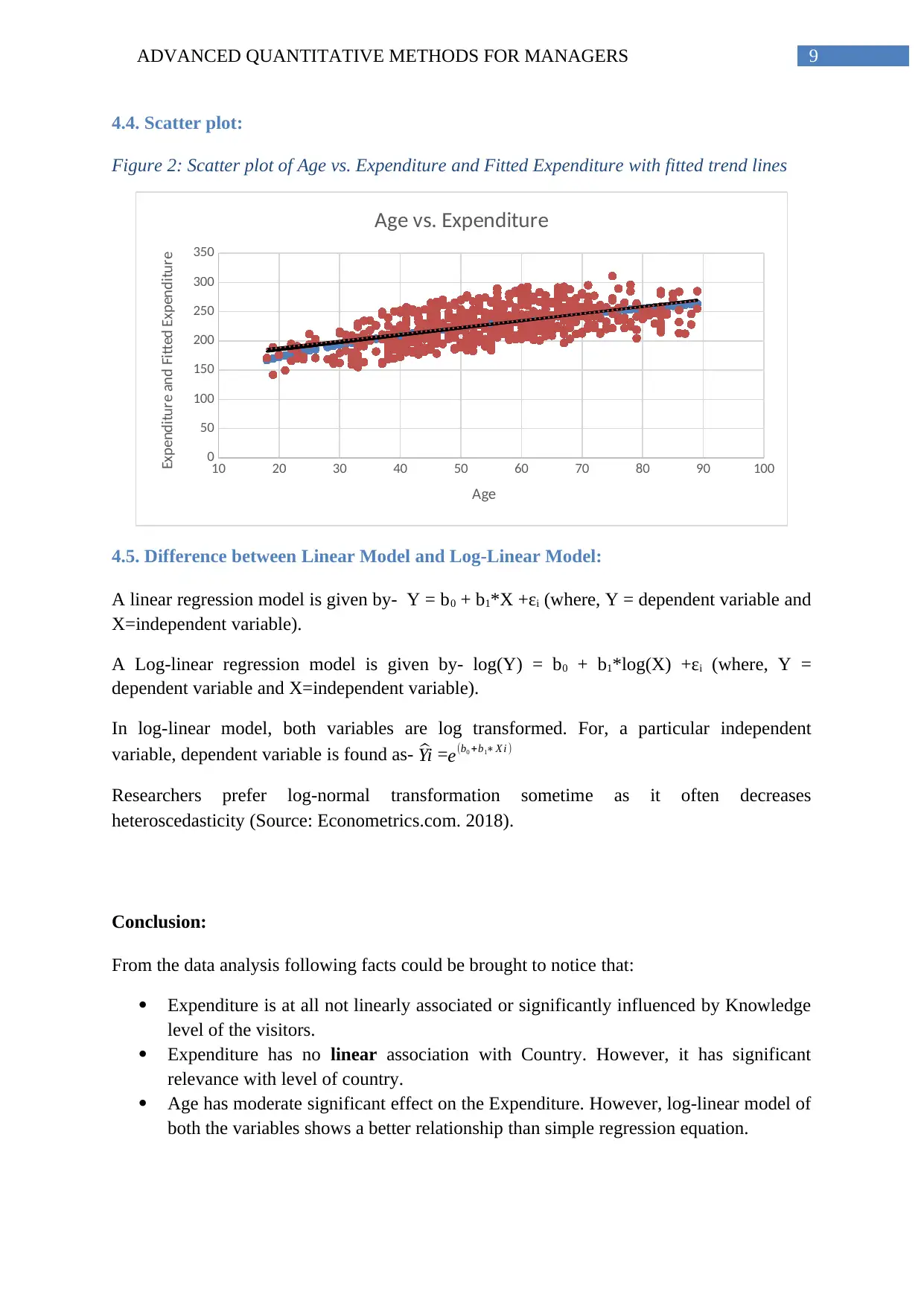
4.4. Scatter plot:
Figure 2: Scatter plot of Age vs. Expenditure and Fitted Expenditure with fitted trend lines
10 20 30 40 50 60 70 80 90 100
0
50
100
150
200
250
300
350
Age vs. Expenditure
Age
Expenditure and Fitted Expenditure
4.5. Difference between Linear Model and Log-Linear Model:
A linear regression model is given by- Y = b0 + b1*X +εi (where, Y = dependent variable and
X=independent variable).
A Log-linear regression model is given by- log(Y) = b0 + b1*log(X) +εi (where, Y =
dependent variable and X=independent variable).
In log-linear model, both variables are log transformed. For, a particular independent
variable, dependent variable is found as- ^Yi =e(b0 +b1∗ X i )
Researchers prefer log-normal transformation sometime as it often decreases
heteroscedasticity (Source: Econometrics.com. 2018).
Conclusion:
From the data analysis following facts could be brought to notice that:
 Expenditure is at all not linearly associated or significantly influenced by Knowledge
level of the visitors.
 Expenditure has no linear association with Country. However, it has significant
relevance with level of country.
 Age has moderate significant effect on the Expenditure. However, log-linear model of
both the variables shows a better relationship than simple regression equation.

10ADVANCED QUANTITATIVE METHODS FOR MANAGERS
References:
Econometrics.com. (2018). Linear vs. log-linear models. Available at:
http://www.econometrics.com/intro/olslog.htm.
Fabozzi, F.J., Focardi, S.M., Rachev, S.T. and Arshanapalli, B.G., 2014. Simple Linear
Regression. The Basics of Financial Econometrics: Tools, Concepts, and Asset Management
Applications, pp.13-39.
Kenbenoit.net. (2018). Cite a Website - Available at:
http://kenbenoit.net/assets/courses/ME104/logmodels2.pdf.
OY, Y., 2015. Simple linear regression. Solutions Manual for Econometrics, p.29.