Relationship between Real GDP and Total Factor Productivity in Different Countries
VerifiedAdded on 2023/05/27
|19
|3706
|227
AI Summary
The article analyzes the growth rate of the economy and the factor productivity of each country. It explains the impact of the global financial crisis on the real GDP growth rate of different economies.
Contribute Materials
Your contribution can guide someone’s learning journey. Share your
documents today.

1
Economics
Economics
Secure Best Marks with AI Grader
Need help grading? Try our AI Grader for instant feedback on your assignments.
2
Table of Contents
Part A.........................................................................................................................................3
Answer 1................................................................................................................................3
Answer 2................................................................................................................................7
Part B........................................................................................................................................11
Effect of increasing government expenditure both on the aggregate demand and aggregate
supply curve.........................................................................................................................11
Part C........................................................................................................................................13
Introduction..........................................................................................................................13
Summary of the Job role......................................................................................................13
Relevancy of the job role.....................................................................................................14
Reflection on the economist interview.................................................................................14
Learning Outcome................................................................................................................15
Conclusion............................................................................................................................15
3
Part A
Answer 1.
1950-01-01
1956-01-01
1962-01-01
1968-01-01
1974-01-01
1980-01-01
1986-01-01
1992-01-01
1998-01-01
2004-01-01
2010-01-01
0.00000
200000.00000
400000.00000
600000.00000
800000.00000
1000000.00000
1200000.00000
0.00000000000
0.20000000000
0.40000000000
0.60000000000
0.80000000000
1.00000000000
1.20000000000
Real GDP
Total Factor Productivity
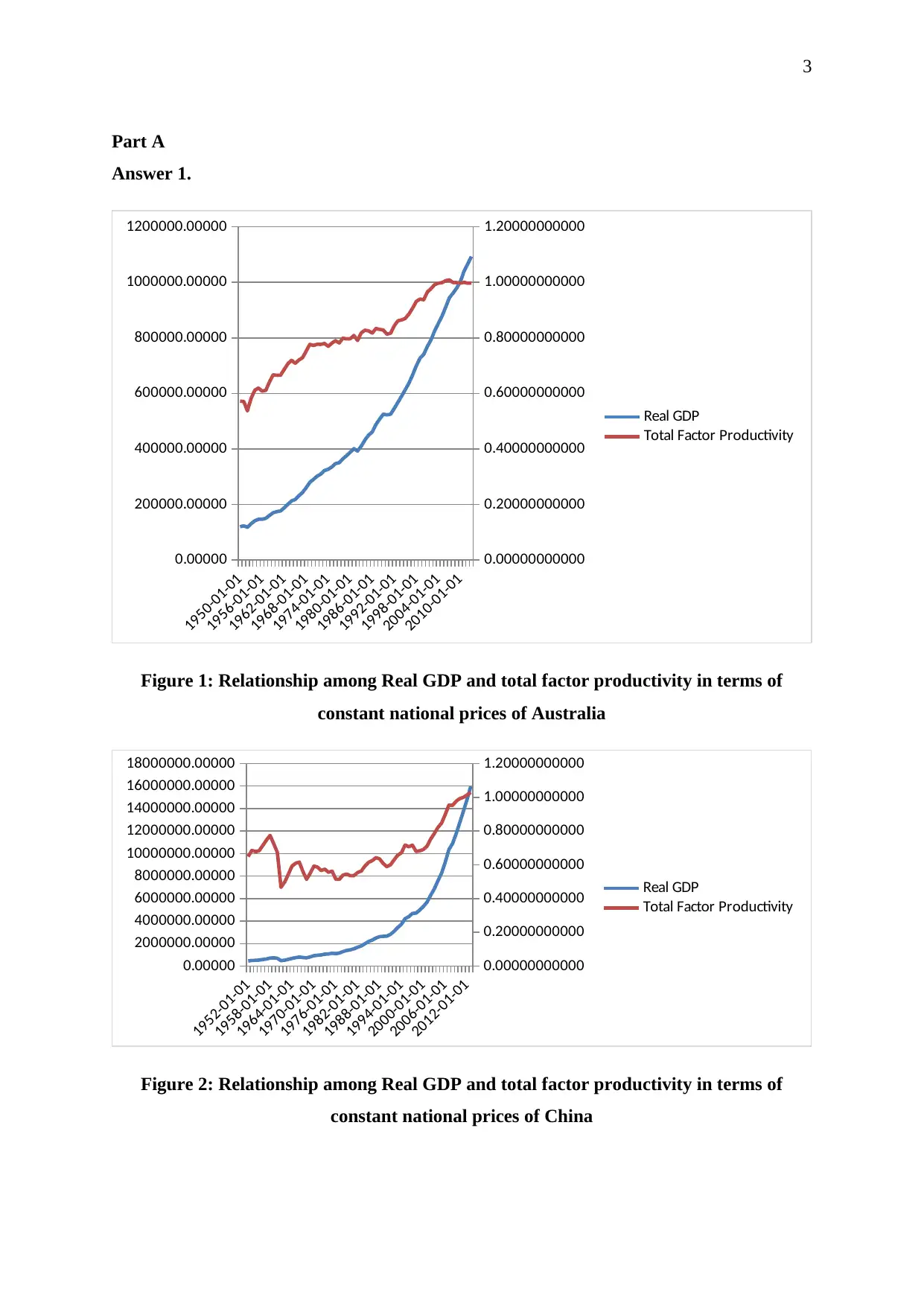
Figure 1: Relationship among Real GDP and total factor productivity in terms of
constant national prices of Australia
1952-01-01
1958-01-01
1964-01-01
1970-01-01
1976-01-01
1982-01-01
1988-01-01
1994-01-01
2000-01-01
2006-01-01
2012-01-01
0.00000
2000000.00000
4000000.00000
6000000.00000
8000000.00000
10000000.00000
12000000.00000
14000000.00000
16000000.00000
18000000.00000
0.00000000000
0.20000000000
0.40000000000
0.60000000000
0.80000000000
1.00000000000
1.20000000000
Real GDP
Total Factor Productivity
Figure 2: Relationship among Real GDP and total factor productivity in terms of
constant national prices of China
4
1950-01-01
1955-01-01
1960-01-01
1965-01-01
1970-01-01
1975-01-01
1980-01-01
1985-01-01
1990-01-01
1995-01-01
2000-01-01
2005-01-01
2010-01-01
0.00000
500000.00000
1000000.00000
1500000.00000
2000000.00000
2500000.00000
3000000.00000
0.00000000000
0.20000000000
0.40000000000
0.60000000000
0.80000000000
1.00000000000
1.20000000000
Real GDP
Total Factor Productivity
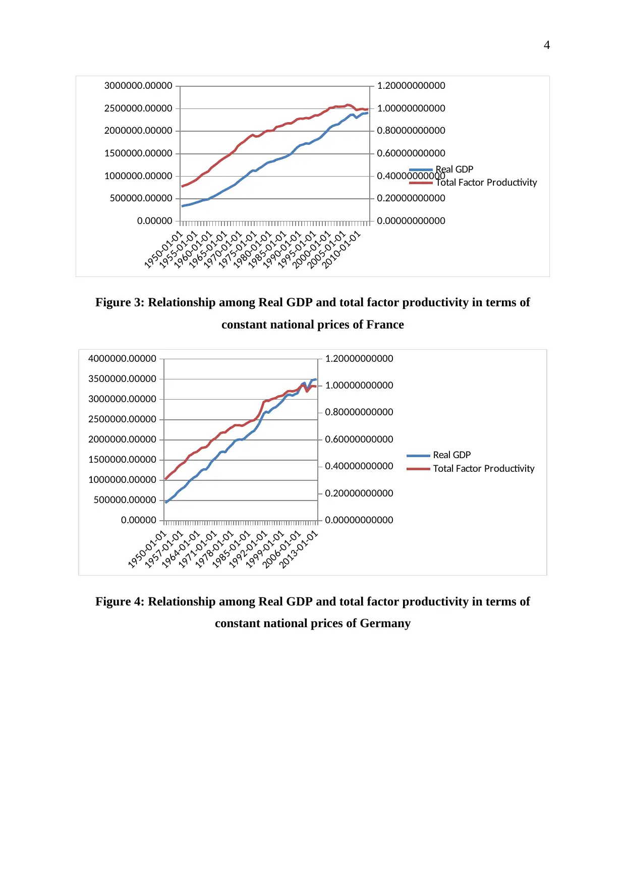
Figure 3: Relationship among Real GDP and total factor productivity in terms of
constant national prices of France
1950-01-01
1957-01-01
1964-01-01
1971-01-01
1978-01-01
1985-01-01
1992-01-01
1999-01-01
2006-01-01
2013-01-01
0.00000
500000.00000
1000000.00000
1500000.00000
2000000.00000
2500000.00000
3000000.00000
3500000.00000
4000000.00000
0.00000000000
0.20000000000
0.40000000000
0.60000000000
0.80000000000
1.00000000000
1.20000000000
Real GDP
Total Factor Productivity
Figure 4: Relationship among Real GDP and total factor productivity in terms of
constant national prices of Germany
1950-01-01
1955-01-01
1960-01-01
1965-01-01
1970-01-01
1975-01-01
1980-01-01
1985-01-01
1990-01-01
1995-01-01
2000-01-01
2005-01-01
2010-01-01
0.00000
500000.00000
1000000.00000
1500000.00000
2000000.00000
2500000.00000
3000000.00000
0.00000000000
0.20000000000
0.40000000000
0.60000000000
0.80000000000
1.00000000000
1.20000000000
Real GDP
Total Factor Productivity
Figure 3: Relationship among Real GDP and total factor productivity in terms of
constant national prices of France
1950-01-01
1957-01-01
1964-01-01
1971-01-01
1978-01-01
1985-01-01
1992-01-01
1999-01-01
2006-01-01
2013-01-01
0.00000
500000.00000
1000000.00000
1500000.00000
2000000.00000
2500000.00000
3000000.00000
3500000.00000
4000000.00000
0.00000000000
0.20000000000
0.40000000000
0.60000000000
0.80000000000
1.00000000000
1.20000000000
Real GDP
Total Factor Productivity
Figure 4: Relationship among Real GDP and total factor productivity in terms of
constant national prices of Germany
Secure Best Marks with AI Grader
Need help grading? Try our AI Grader for instant feedback on your assignments.
5
1950-01-01
1956-01-01
1962-01-01
1968-01-01
1974-01-01
1980-01-01
1986-01-01
1992-01-01
1998-01-01
2004-01-01
2010-01-01
0.00000
500000.00000
1000000.00000
1500000.00000
2000000.00000
2500000.00000
3000000.00000
3500000.00000
4000000.00000
4500000.00000
5000000.00000
0.00000000000
0.20000000000
0.40000000000
0.60000000000
0.80000000000
1.00000000000
1.20000000000
1.40000000000
Real GDP
Total Factor Productivity
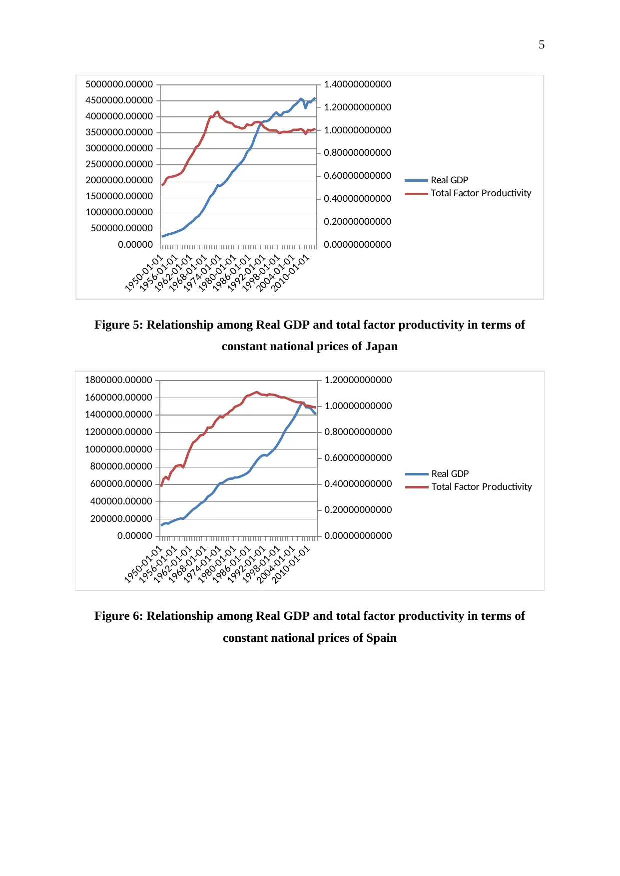
Figure 5: Relationship among Real GDP and total factor productivity in terms of
constant national prices of Japan
1950-01-01
1956-01-01
1962-01-01
1968-01-01
1974-01-01
1980-01-01
1986-01-01
1992-01-01
1998-01-01
2004-01-01
2010-01-01
0.00000
200000.00000
400000.00000
600000.00000
800000.00000
1000000.00000
1200000.00000
1400000.00000
1600000.00000
1800000.00000
0.00000000000
0.20000000000
0.40000000000
0.60000000000
0.80000000000
1.00000000000
1.20000000000
Real GDP
Total Factor Productivity
Figure 6: Relationship among Real GDP and total factor productivity in terms of
constant national prices of Spain
1950-01-01
1956-01-01
1962-01-01
1968-01-01
1974-01-01
1980-01-01
1986-01-01
1992-01-01
1998-01-01
2004-01-01
2010-01-01
0.00000
500000.00000
1000000.00000
1500000.00000
2000000.00000
2500000.00000
3000000.00000
3500000.00000
4000000.00000
4500000.00000
5000000.00000
0.00000000000
0.20000000000
0.40000000000
0.60000000000
0.80000000000
1.00000000000
1.20000000000
1.40000000000
Real GDP
Total Factor Productivity
Figure 5: Relationship among Real GDP and total factor productivity in terms of
constant national prices of Japan
1950-01-01
1956-01-01
1962-01-01
1968-01-01
1974-01-01
1980-01-01
1986-01-01
1992-01-01
1998-01-01
2004-01-01
2010-01-01
0.00000
200000.00000
400000.00000
600000.00000
800000.00000
1000000.00000
1200000.00000
1400000.00000
1600000.00000
1800000.00000
0.00000000000
0.20000000000
0.40000000000
0.60000000000
0.80000000000
1.00000000000
1.20000000000
Real GDP
Total Factor Productivity
Figure 6: Relationship among Real GDP and total factor productivity in terms of
constant national prices of Spain
6
1950-01-01
1955-01-01
1960-01-01
1965-01-01
1970-01-01
1975-01-01
1980-01-01
1985-01-01
1990-01-01
1995-01-01
2000-01-01
2005-01-01
2010-01-01
0
200000
400000
600000
800000
1000000
1200000
1400000
1600000
1800000
2000000
0.00000000000
0.20000000000
0.40000000000
0.60000000000
0.80000000000
1.00000000000
1.20000000000
Real GDP
Total Factor Productivity
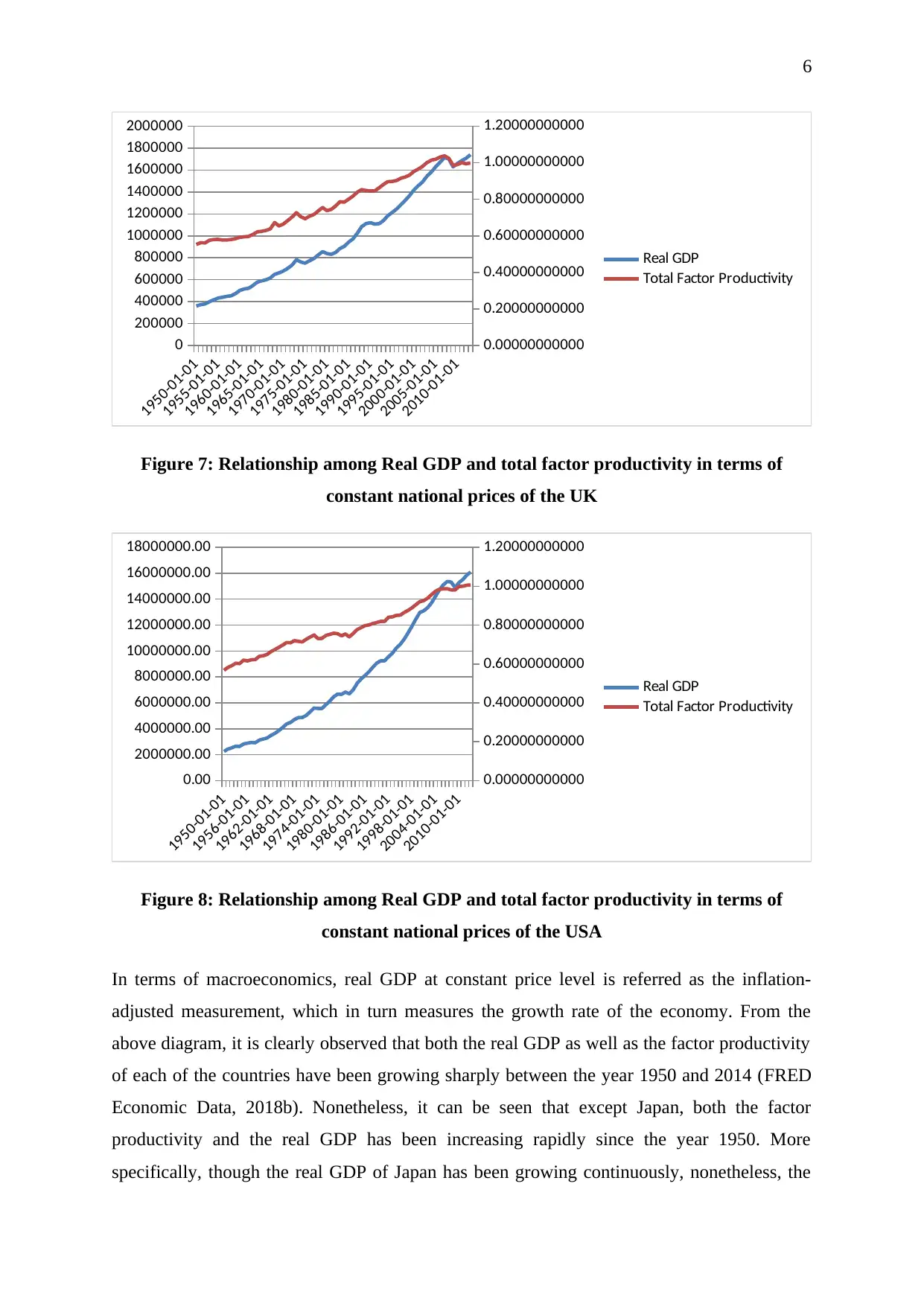
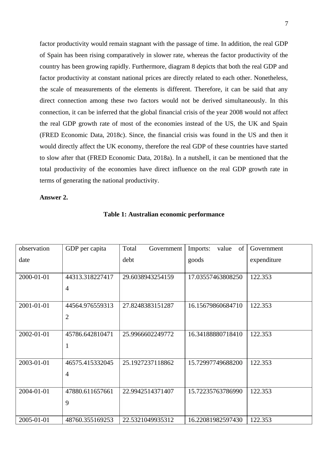
Figure 7: Relationship among Real GDP and total factor productivity in terms of
constant national prices of the UK
1950-01-01
1956-01-01
1962-01-01
1968-01-01
1974-01-01
1980-01-01
1986-01-01
1992-01-01
1998-01-01
2004-01-01
2010-01-01
0.00
2000000.00
4000000.00
6000000.00
8000000.00
10000000.00
12000000.00
14000000.00
16000000.00
18000000.00
0.00000000000
0.20000000000
0.40000000000
0.60000000000
0.80000000000
1.00000000000
1.20000000000
Real GDP
Total Factor Productivity
Figure 8: Relationship among Real GDP and total factor productivity in terms of
constant national prices of the USA
In terms of macroeconomics, real GDP at constant price level is referred as the inflation-
adjusted measurement, which in turn measures the growth rate of the economy. From the
above diagram, it is clearly observed that both the real GDP as well as the factor productivity
of each of the countries have been growing sharply between the year 1950 and 2014 (FRED
Economic Data, 2018b). Nonetheless, it can be seen that except Japan, both the factor
productivity and the real GDP has been increasing rapidly since the year 1950. More
specifically, though the real GDP of Japan has been growing continuously, nonetheless, the
1950-01-01
1955-01-01
1960-01-01
1965-01-01
1970-01-01
1975-01-01
1980-01-01
1985-01-01
1990-01-01
1995-01-01
2000-01-01
2005-01-01
2010-01-01
0
200000
400000
600000
800000
1000000
1200000
1400000
1600000
1800000
2000000
0.00000000000
0.20000000000
0.40000000000
0.60000000000
0.80000000000
1.00000000000
1.20000000000
Real GDP
Total Factor Productivity
Figure 7: Relationship among Real GDP and total factor productivity in terms of
constant national prices of the UK
1950-01-01
1956-01-01
1962-01-01
1968-01-01
1974-01-01
1980-01-01
1986-01-01
1992-01-01
1998-01-01
2004-01-01
2010-01-01
0.00
2000000.00
4000000.00
6000000.00
8000000.00
10000000.00
12000000.00
14000000.00
16000000.00
18000000.00
0.00000000000
0.20000000000
0.40000000000
0.60000000000
0.80000000000
1.00000000000
1.20000000000
Real GDP
Total Factor Productivity
Figure 8: Relationship among Real GDP and total factor productivity in terms of
constant national prices of the USA
In terms of macroeconomics, real GDP at constant price level is referred as the inflation-
adjusted measurement, which in turn measures the growth rate of the economy. From the
above diagram, it is clearly observed that both the real GDP as well as the factor productivity
of each of the countries have been growing sharply between the year 1950 and 2014 (FRED
Economic Data, 2018b). Nonetheless, it can be seen that except Japan, both the factor
productivity and the real GDP has been increasing rapidly since the year 1950. More
specifically, though the real GDP of Japan has been growing continuously, nonetheless, the
7
factor productivity would remain stagnant with the passage of time. In addition, the real GDP
of Spain has been rising comparatively in slower rate, whereas the factor productivity of the
country has been growing rapidly. Furthermore, diagram 8 depicts that both the real GDP and
factor productivity at constant national prices are directly related to each other. Nonetheless,
the scale of measurements of the elements is different. Therefore, it can be said that any
direct connection among these two factors would not be derived simultaneously. In this
connection, it can be inferred that the global financial crisis of the year 2008 would not affect
the real GDP growth rate of most of the economies instead of the US, the UK and Spain
(FRED Economic Data, 2018c). Since, the financial crisis was found in the US and then it
would directly affect the UK economy, therefore the real GDP of these countries have started
to slow after that (FRED Economic Data, 2018a). In a nutshell, it can be mentioned that the
total productivity of the economies have direct influence on the real GDP growth rate in
terms of generating the national productivity.
Answer 2.
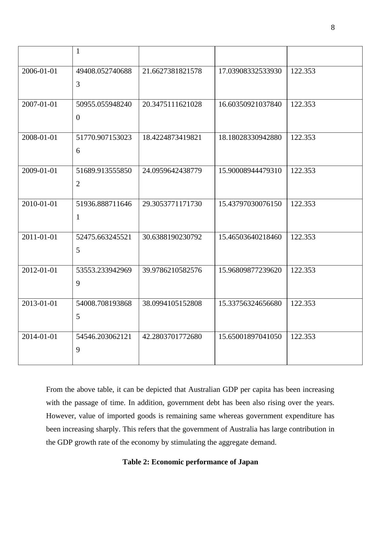
Table 1: Australian economic performance
observation
date
GDP per capita Total Government
debt
Imports: value of
goods
Government
expenditure
2000-01-01 44313.318227417
4
29.6038943254159 17.03557463808250 122.353
2001-01-01 44564.976559313
2
27.8248383151287 16.15679860684710 122.353
2002-01-01 45786.642810471
1
25.9966602249772 16.34188880718410 122.353
2003-01-01 46575.415332045
4
25.1927237118862 15.72997749688200 122.353
2004-01-01 47880.611657661
9
22.9942514371407 15.72235763786990 122.353
2005-01-01 48760.355169253 22.5321049935312 16.22081982597430 122.353
Paraphrase This Document
Need a fresh take? Get an instant paraphrase of this document with our AI Paraphraser
8
1
2006-01-01 49408.052740688
3
21.6627381821578 17.03908332533930 122.353
2007-01-01 50955.055948240
0
20.3475111621028 16.60350921037840 122.353
2008-01-01 51770.907153023
6
18.4224873419821 18.18028330942880 122.353
2009-01-01 51689.913555850
2
24.0959642438779 15.90008944479310 122.353
2010-01-01 51936.888711646
1
29.3053771171730 15.43797030076150 122.353
2011-01-01 52475.663245521
5
30.6388190230792 15.46503640218460 122.353
2012-01-01 53553.233942969
9
39.9786210582576 15.96809877239620 122.353
2013-01-01 54008.708193868
5
38.0994105152808 15.33756324656680 122.353
2014-01-01 54546.203062121
9
42.2803701772680 15.65001897041050 122.353
From the above table, it can be depicted that Australian GDP per capita has been increasing
with the passage of time. In addition, government debt has been also rising over the years.
However, value of imported goods is remaining same whereas government expenditure has
been increasing sharply. This refers that the government of Australia has large contribution in
the GDP growth rate of the economy by stimulating the aggregate demand.
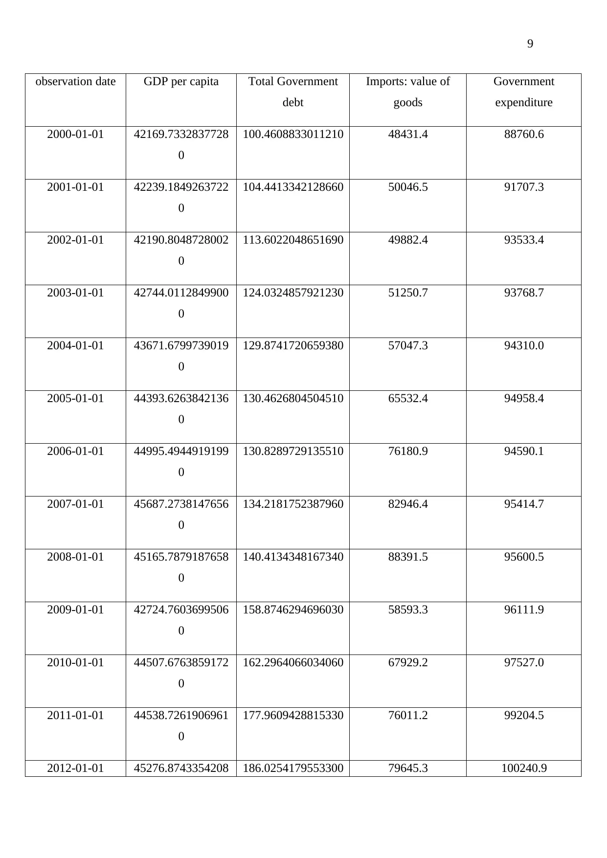
Table 2: Economic performance of Japan
1
2006-01-01 49408.052740688
3
21.6627381821578 17.03908332533930 122.353
2007-01-01 50955.055948240
0
20.3475111621028 16.60350921037840 122.353
2008-01-01 51770.907153023
6
18.4224873419821 18.18028330942880 122.353
2009-01-01 51689.913555850
2
24.0959642438779 15.90008944479310 122.353
2010-01-01 51936.888711646
1
29.3053771171730 15.43797030076150 122.353
2011-01-01 52475.663245521
5
30.6388190230792 15.46503640218460 122.353
2012-01-01 53553.233942969
9
39.9786210582576 15.96809877239620 122.353
2013-01-01 54008.708193868
5
38.0994105152808 15.33756324656680 122.353
2014-01-01 54546.203062121
9
42.2803701772680 15.65001897041050 122.353
From the above table, it can be depicted that Australian GDP per capita has been increasing
with the passage of time. In addition, government debt has been also rising over the years.
However, value of imported goods is remaining same whereas government expenditure has
been increasing sharply. This refers that the government of Australia has large contribution in
the GDP growth rate of the economy by stimulating the aggregate demand.
Table 2: Economic performance of Japan
9
observation date GDP per capita Total Government
debt
Imports: value of
goods
Government
expenditure
2000-01-01 42169.7332837728
0
100.4608833011210 48431.4 88760.6
2001-01-01 42239.1849263722
0
104.4413342128660 50046.5 91707.3
2002-01-01 42190.8048728002
0
113.6022048651690 49882.4 93533.4
2003-01-01 42744.0112849900
0
124.0324857921230 51250.7 93768.7
2004-01-01 43671.6799739019
0
129.8741720659380 57047.3 94310.0
2005-01-01 44393.6263842136
0
130.4626804504510 65532.4 94958.4
2006-01-01 44995.4944919199
0
130.8289729135510 76180.9 94590.1
2007-01-01 45687.2738147656
0
134.2181752387960 82946.4 95414.7
2008-01-01 45165.7879187658
0
140.4134348167340 88391.5 95600.5
2009-01-01 42724.7603699506
0
158.8746294696030 58593.3 96111.9
2010-01-01 44507.6763859172
0
162.2964066034060 67929.2 97527.0
2011-01-01 44538.7261906961
0
177.9609428815330 76011.2 99204.5
2012-01-01 45276.8743354208 186.0254179553300 79645.3 100240.9
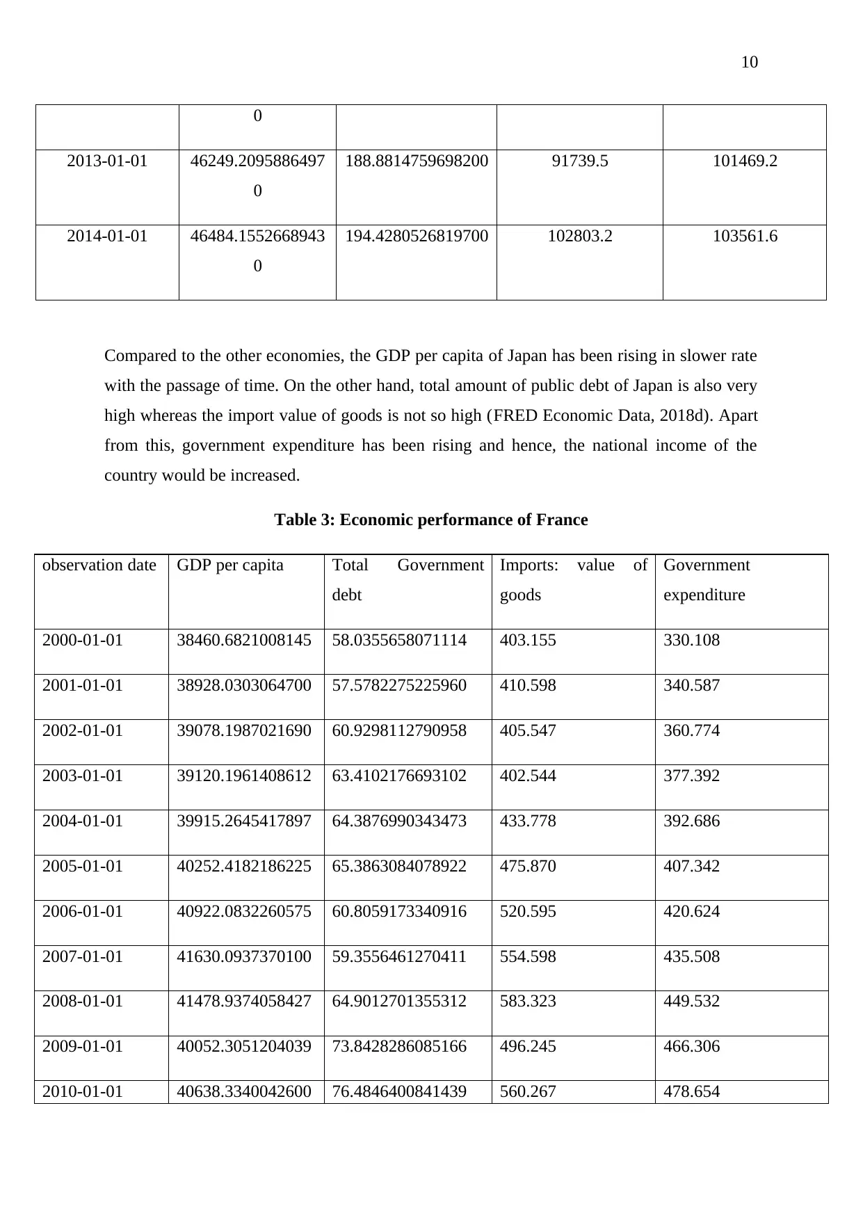
10
0
2013-01-01 46249.2095886497
0
188.8814759698200 91739.5 101469.2
2014-01-01 46484.1552668943
0
194.4280526819700 102803.2 103561.6
Compared to the other economies, the GDP per capita of Japan has been rising in slower rate
with the passage of time. On the other hand, total amount of public debt of Japan is also very
high whereas the import value of goods is not so high (FRED Economic Data, 2018d). Apart
from this, government expenditure has been rising and hence, the national income of the
country would be increased.
Table 3: Economic performance of France
observation date GDP per capita Total Government
debt
Imports: value of
goods
Government
expenditure
2000-01-01 38460.6821008145 58.0355658071114 403.155 330.108
2001-01-01 38928.0303064700 57.5782275225960 410.598 340.587
2002-01-01 39078.1987021690 60.9298112790958 405.547 360.774
2003-01-01 39120.1961408612 63.4102176693102 402.544 377.392
2004-01-01 39915.2645417897 64.3876990343473 433.778 392.686
2005-01-01 40252.4182186225 65.3863084078922 475.870 407.342
2006-01-01 40922.0832260575 60.8059173340916 520.595 420.624
2007-01-01 41630.0937370100 59.3556461270411 554.598 435.508
2008-01-01 41478.9374058427 64.9012701355312 583.323 449.532
2009-01-01 40052.3051204039 73.8428286085166 496.245 466.306
2010-01-01 40638.3340042600 76.4846400841439 560.267 478.654
0
2013-01-01 46249.2095886497
0
188.8814759698200 91739.5 101469.2
2014-01-01 46484.1552668943
0
194.4280526819700 102803.2 103561.6
Compared to the other economies, the GDP per capita of Japan has been rising in slower rate
with the passage of time. On the other hand, total amount of public debt of Japan is also very
high whereas the import value of goods is not so high (FRED Economic Data, 2018d). Apart
from this, government expenditure has been rising and hence, the national income of the
country would be increased.
Table 3: Economic performance of France
observation date GDP per capita Total Government
debt
Imports: value of
goods
Government
expenditure
2000-01-01 38460.6821008145 58.0355658071114 403.155 330.108
2001-01-01 38928.0303064700 57.5782275225960 410.598 340.587
2002-01-01 39078.1987021690 60.9298112790958 405.547 360.774
2003-01-01 39120.1961408612 63.4102176693102 402.544 377.392
2004-01-01 39915.2645417897 64.3876990343473 433.778 392.686
2005-01-01 40252.4182186225 65.3863084078922 475.870 407.342
2006-01-01 40922.0832260575 60.8059173340916 520.595 420.624
2007-01-01 41630.0937370100 59.3556461270411 554.598 435.508
2008-01-01 41478.9374058427 64.9012701355312 583.323 449.532
2009-01-01 40052.3051204039 73.8428286085166 496.245 466.306
2010-01-01 40638.3340042600 76.4846400841439 560.267 478.654
Secure Best Marks with AI Grader
Need help grading? Try our AI Grader for instant feedback on your assignments.
11
2011-01-01 41283.1481006903 79.7061988535821 625.111 488.749
2012-01-01 41158.8849843807 88.9999611869882 637.064 500.279
2013-01-01 41183.5109594260 89.7922993718018 643.610 510.491
2014-01-01 41374.7612490442 97.6656365288095 662.388 518.651
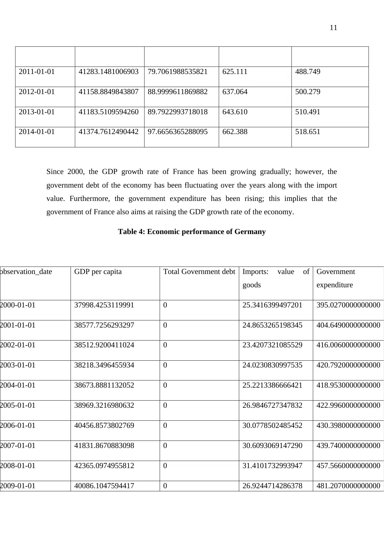
Since 2000, the GDP growth rate of France has been growing gradually; however, the
government debt of the economy has been fluctuating over the years along with the import
value. Furthermore, the government expenditure has been rising; this implies that the
government of France also aims at raising the GDP growth rate of the economy.
Table 4: Economic performance of Germany
observation_date GDP per capita Total Government debt Imports: value of
goods
Government
expenditure
2000-01-01 37998.4253119991 0 25.3416399497201 395.0270000000000
2001-01-01 38577.7256293297 0 24.8653265198345 404.6490000000000
2002-01-01 38512.9200411024 0 23.4207321085529 416.0060000000000
2003-01-01 38218.3496455934 0 24.0230830997535 420.7920000000000
2004-01-01 38673.8881132052 0 25.2213386666421 418.9530000000000
2005-01-01 38969.3216980632 0 26.9846727347832 422.9960000000000
2006-01-01 40456.8573802769 0 30.0778502485452 430.3980000000000
2007-01-01 41831.8670883098 0 30.6093069147290 439.7400000000000
2008-01-01 42365.0974955812 0 31.4101732993947 457.5660000000000
2009-01-01 40086.1047594417 0 26.9244714286378 481.2070000000000
12
2010-01-01 41785.5569125540 0 30.6746510777566 493.3360000000000
2011-01-01 44125.3314116503 0 33.1773931675684 505.6910000000000
2012-01-01 44259.2599053983 0 32.5643076177782 519.7130000000000
2013-01-01 44354.7368865267 0 31.4182617638523 542.8530000000000
2014-01-01 45022.5653486423 0 30.8567350338028 563.9620000000000
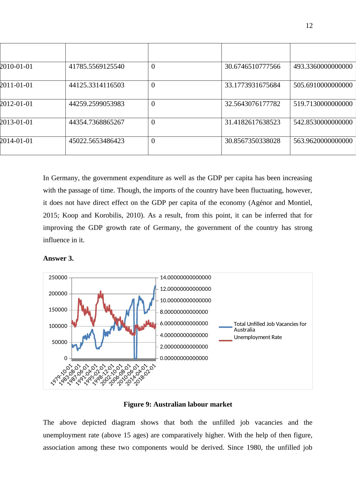
In Germany, the government expenditure as well as the GDP per capita has been increasing
with the passage of time. Though, the imports of the country have been fluctuating, however,
it does not have direct effect on the GDP per capita of the economy (Agénor and Montiel,
2015; Koop and Korobilis, 2010). As a result, from this point, it can be inferred that for
improving the GDP growth rate of Germany, the government of the country has strong
influence in it.
Answer 3.
1979-10-01
1983-08-01
1987-06-01
1991-04-01
1995-02-01
1998-12-01
2002-10-01
2006-08-01
2010-06-01
2014-04-01
2018-02-01
0
50000
100000
150000
200000
250000
0.00000000000000
2.00000000000000
4.00000000000000
6.00000000000000
8.00000000000000
10.00000000000000
12.00000000000000
14.00000000000000
Total Unfilled Job Vacancies for
Australia
Unemployment Rate
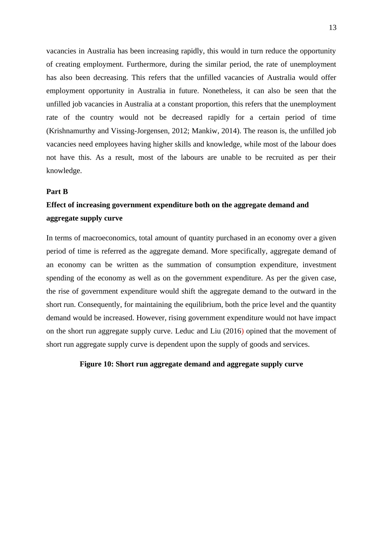
Figure 9: Australian labour market
The above depicted diagram shows that both the unfilled job vacancies and the
unemployment rate (above 15 ages) are comparatively higher. With the help of then figure,
association among these two components would be derived. Since 1980, the unfilled job
13
vacancies in Australia has been increasing rapidly, this would in turn reduce the opportunity
of creating employment. Furthermore, during the similar period, the rate of unemployment
has also been decreasing. This refers that the unfilled vacancies of Australia would offer
employment opportunity in Australia in future. Nonetheless, it can also be seen that the
unfilled job vacancies in Australia at a constant proportion, this refers that the unemployment
rate of the country would not be decreased rapidly for a certain period of time
(Krishnamurthy and Vissing-Jorgensen, 2012; Mankiw, 2014). The reason is, the unfilled job
vacancies need employees having higher skills and knowledge, while most of the labour does
not have this. As a result, most of the labours are unable to be recruited as per their
knowledge.
Part B
Effect of increasing government expenditure both on the aggregate demand and
aggregate supply curve
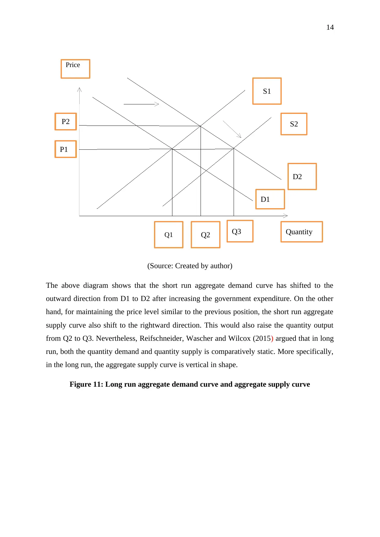
In terms of macroeconomics, total amount of quantity purchased in an economy over a given
period of time is referred as the aggregate demand. More specifically, aggregate demand of
an economy can be written as the summation of consumption expenditure, investment
spending of the economy as well as on the government expenditure. As per the given case,
the rise of government expenditure would shift the aggregate demand to the outward in the
short run. Consequently, for maintaining the equilibrium, both the price level and the quantity
demand would be increased. However, rising government expenditure would not have impact
on the short run aggregate supply curve. Leduc and Liu (2016) opined that the movement of
short run aggregate supply curve is dependent upon the supply of goods and services.
Figure 10: Short run aggregate demand and aggregate supply curve
Paraphrase This Document
Need a fresh take? Get an instant paraphrase of this document with our AI Paraphraser
S1
Price
Quantity
D2
D1
Q2Q1
P2
P1
S2
Q3
14
(Source: Created by author)
The above diagram shows that the short run aggregate demand curve has shifted to the
outward direction from D1 to D2 after increasing the government expenditure. On the other
hand, for maintaining the price level similar to the previous position, the short run aggregate
supply curve also shift to the rightward direction. This would also raise the quantity output
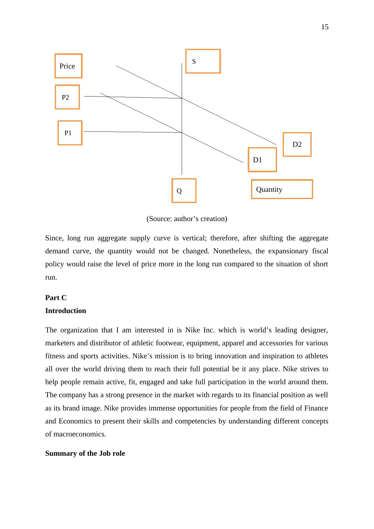
from Q2 to Q3. Nevertheless, Reifschneider, Wascher and Wilcox (2015) argued that in long
run, both the quantity demand and quantity supply is comparatively static. More specifically,
in the long run, the aggregate supply curve is vertical in shape.
Figure 11: Long run aggregate demand curve and aggregate supply curve
D2
D1
Quantity
Price S
Q
P2
P1
15
(Source: author’s creation)
Since, long run aggregate supply curve is vertical; therefore, after shifting the aggregate
demand curve, the quantity would not be changed. Nonetheless, the expansionary fiscal
policy would raise the level of price more in the long run compared to the situation of short
run.
Part C
Introduction
The organization that I am interested in is Nike Inc. which is world’s leading designer,
marketers and distributor of athletic footwear, equipment, apparel and accessories for various
fitness and sports activities. Nike’s mission is to bring innovation and inspiration to athletes
all over the world driving them to reach their full potential be it any place. Nike strives to
help people remain active, fit, engaged and take full participation in the world around them.
The company has a strong presence in the market with regards to its financial position as well
as its brand image. Nike provides immense opportunities for people from the field of Finance
and Economics to present their skills and competencies by understanding different concepts
of macroeconomics.
Summary of the Job role

16
Nike recently posted an opening in its official career website for the position of Finance
Manager which suits my requirement. I would be interested in taking the opportunity of
applying for this position after the completion of my degree in finance. The role of a Finance
Manger will require me to participate in Finance projects of Nike by doing in-depth research,
analysis and benchmarking my performance, and focus on next step recommendations. This
will also require me to tale initiative across different departments, participate in functional
discussions, and contribute toward business unit planning. The job role demands the
preparation and timely distribution of financial reports including making strategic plans
towards budget planning and forecasting of financial data. The job will also require
achievement of the learning outcomes of the Economics Learning Standards for Bachelor
graduate students (Economics Learning Standards for Australian Higher Education, 2018). I
have continued to gain confidence on my strengths and skills which focuses on
accomplishing given targets within deadlines by use of my practical knowledge.
However, I would like to make room for certain improvements in my knowledge in the field
of finance and economics. I would also like to upgrade my skills through constant learning
and hope to show recruiters by my abilities to fulfil the requirements of the job role.
Relevancy of the job role
The given job position aligns with my requirements and interests in financial analysis and
study of economics. It aligns with my existing skills and compassion for the field of finance.
My career personality results reflect that I am a problem solver and understand the
importance of self-management. This will allow me to identify relevant solutions to various
commerce related issues along with be accountable for my own actions and make continuous
improvements in identifying gaps in my performance and plan for future developments. This
would allow me to utilize my skills and competencies for the achievement of both personal
and organizational objectives after deriving relevant knowledge from my course.
Reflection on the economist interview
The Economist Informational interview video focused on the study of finance and economics
helps in analysing the current market and make further improvements for its betterment. The
understood from the interview that the theories of finance and economics are vast and is
definitely derive the benefits of taking the mentioned job role. The speaker’s words motivated
me to apply the relevant theories learned by me in the course. I understood the importance of
Secure Best Marks with AI Grader
Need help grading? Try our AI Grader for instant feedback on your assignments.

17
understanding the concepts of finance and this can be improved by taking up internships to
gain practical experience. The real understanding of the concepts can also be possible by the
achievement of practical knowledge of the concepts learned. I started focusing more on the
future prospects I will derive from this job position.
Learning Outcome
I want my strengths and knowledge to become my pillars of success. Although I am making
improvements in my overall personal development, I would also like to improve my
leadership qualities and quality in performance. I want to identify relevant techniques that
facilitate my need of better analytical and leadership skills. The actions that I can take are to
take up internships and courses, attend conferences and financial talks from industry experts
to improve my knowledge on finance as well as economics.
Conclusion
My dream to work as a Finance Manger will be accomplished after successfully completing
my course. I wish to improve in near future from my own mistakes, continuous efforts
towards building my overall personality and upgrading my knowledge in the field of finance
and economics.
18
Reference List
Agénor, P.R. and Montiel, P.J., 2015. Development macroeconomics. Princeton University
Press.
Economics Learning Standards for Australian Higher Education, 2018. Overview.
[online]Available at:
http://www.weebly.com/uploads/1/3/7/6/13761320/146_13_economics_learning_stds_c17_w
eb.pdf [Accessed 18 January 2019]
FRED Economic Data, 2018a. Harmonized Unemployment Rate: Total: All Persons for
Australia. [online] Available at < https://fred.stlouisfed.org/series/LRHUTTTTAUQ156N>
[Accessed 18 Jan 2019].
FRED Economic Data, 2018b. Real GDP at Constant National Prices for United States.
[online] Available at <https://fred.stlouisfed.org/series/RGDPNAUSA666NRUG> [Accessed
18 Jan 2019].
FRED Economic Data, 2018c. Real GDP at Constant National Prices for Japan. [online]
Available at <https://fred.stlouisfed.org/series/RGDPNAJPA666NRUG> [Accessed 18 Jan
2019].
FRED Economic Data, 2018d. Real GDP at Constant National Prices for Spain. [online]
Available at <https://fred.stlouisfed.org/series/RGDPNAESA666NRUG> [Accessed 18 Jan
2019].
Koop, G. and Korobilis, D., 2010. Bayesian multivariate time series methods for empirical
macroeconomics. Foundations and Trends in Econometrics, 3(4), pp.267-358.
Krishnamurthy, A. and Vissing-Jorgensen, A., 2012. The aggregate demand for treasury debt.
Journal of Political Economy, 120(2), pp.233-267.
Leduc, S. and Liu, Z., 2016. Uncertainty shocks are aggregate demand shocks. Journal of
Monetary Economics, 82, pp.20-35.
Mankiw, N.G., 2014. Principles of macroeconomics. Cengage Learning.

19
Reifschneider, D., Wascher, W. and Wilcox, D., 2015. Aggregate supply in the United States:
recent developments and implications for the conduct of monetary policy. IMF Economic
Review, 63(1), pp.71-109.
Reifschneider, D., Wascher, W. and Wilcox, D., 2015. Aggregate supply in the United States:
recent developments and implications for the conduct of monetary policy. IMF Economic
Review, 63(1), pp.71-109.
1 out of 19
Related Documents
Your All-in-One AI-Powered Toolkit for Academic Success.
+13062052269
info@desklib.com
Available 24*7 on WhatsApp / Email
![[object Object]](/_next/static/media/star-bottom.7253800d.svg)
Unlock your academic potential
© 2024 | Zucol Services PVT LTD | All rights reserved.


