Statistical Quality Control Analysis

This solved assignment explores the concept of statistical quality control with two distinct problems. The first involves calculating control limits for labor time using a given mean and standard deviation. It then compares three alternative procedures with different sample sizes to determine the narrowest control limits. The second problem examines occupational sick days in company A, comparing their data to the national average through a one-sample t-test. This includes formulating hypotheses, calculating the test statistic, and interpreting the results within the context of the company's claim.

Running Head: DECISION MAKING
Decision Making
Name of the Student
Name of the University
Author Note

1DECISION MAKING
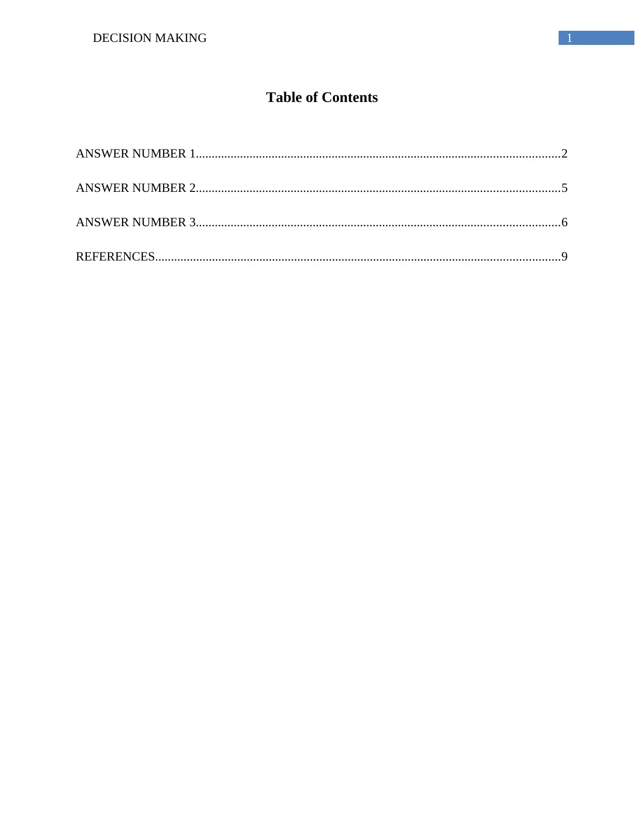
Table of Contents
ANSWER NUMBER 1...................................................................................................................2
ANSWER NUMBER 2...................................................................................................................5
ANSWER NUMBER 3...................................................................................................................6
REFERENCES................................................................................................................................9

2DECISION MAKING
ANSWER NUMBER 1
a) In certain situations, real numbers are attached along with the elementary events that can
be obtained by performing a random experiment. The elementary events that can be obtained by
conducting a random experiment is known as the sample space. As an example, tossing of a coin
can be considered. Let the number 1 be assigned with the appearance of a tail and 0 be assigned
with the appearance of head. This is how a function is defined on a sample space. A (real valued)
function defined on the sample space is known as the random variable or a stochastic variable.
To each value of a random variable X, there corresponds a definite probability.
Random variable can be classified into two types – discrete random variables and
continuous random variables (Miller & Miller, 2015).
A random variable, which takes a finite number of values or a countably infinite number
of values, is known as a discrete random variable. The number of misprints in a page of book is
an example of a discrete random variable.
A random variable is said to be continuous if it assumes uncountably infinite number of
values. For example, the waiting time in a bus stop for the arrival of a bus is a continuous
random variable.
b) The term expected value of a random variable means the value predicted for the
respective random variable. It is denoted by E(X) and serves as a measure of central tendency of
the probability distribution of X. It is usually defines as the sum of the values of the random

3DECISION MAKING
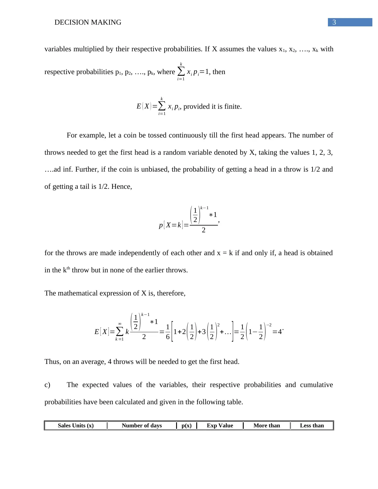
variables multiplied by their respective probabilities. If X assumes the values x1, x2, …., xk with
respective probabilities p1, p2, …., pk, where ∑
i=1
k
xi pi=1, then
E ( X ) =∑
i=1
k
xi pi, provided it is finite.
For example, let a coin be tossed continuously till the first head appears. The number of
throws needed to get the first head is a random variable denoted by X, taking the values 1, 2, 3,
….ad inf. Further, if the coin is unbiased, the probability of getting a head in a throw is 1/2 and
of getting a tail is 1/2. Hence,
p [ X=k ] = ( 1
2 )
k−1
∗1
2
,
for the throws are made independently of each other and x = k if and only if, a head is obtained
in the kth throw but in none of the earlier throws.
The mathematical expression of X is, therefore,
E [ X ] =∑
k =1
∞
k ( 1
2 ) k−1
∗1
2 = 1
6 [ 1+2 ( 1
2 ) +3 ( 1
2 )
2
+ … ]= 1
2 ( 1− 1
2 )
−2
=4.
Thus, on an average, 4 throws will be needed to get the first head.
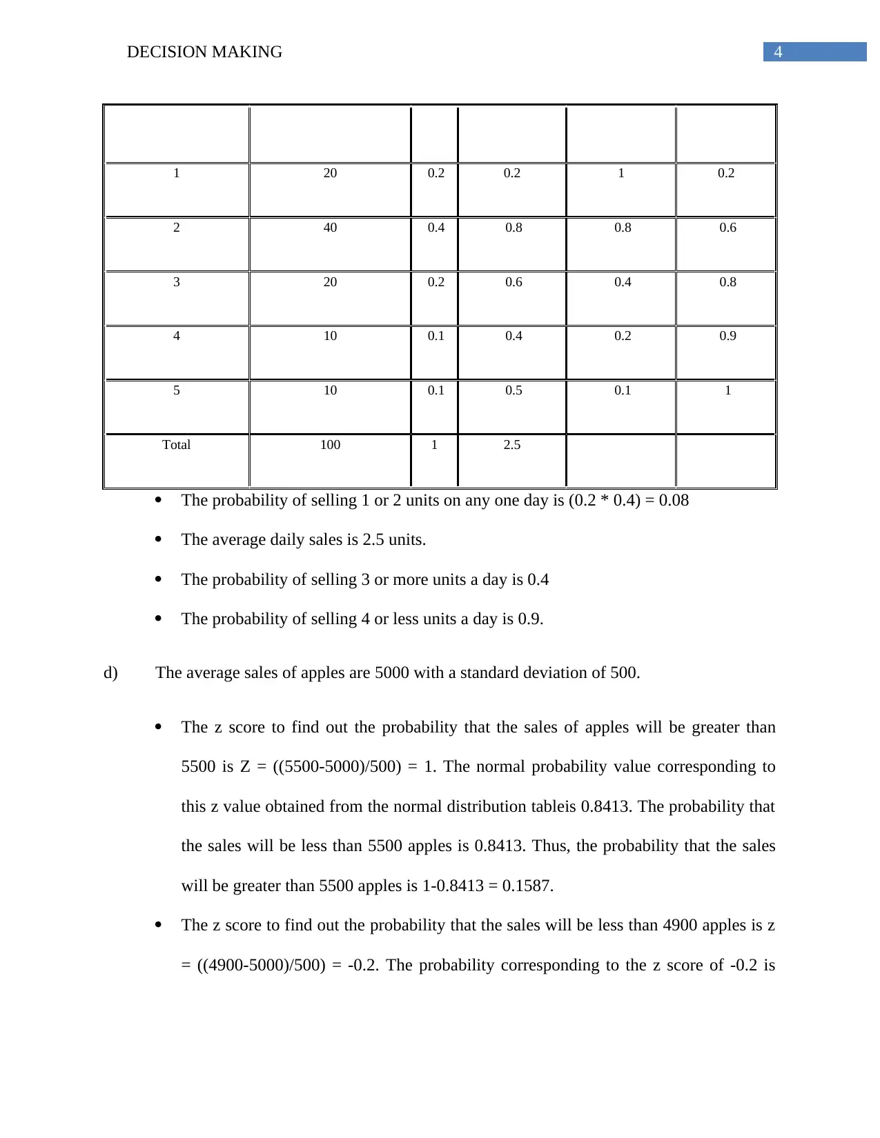
c) The expected values of the variables, their respective probabilities and cumulative
probabilities have been calculated and given in the following table.
Sales Units (x) Number of days p(x) Exp Value More than Less than

4DECISION MAKING
1 20 0.2 0.2 1 0.2
2 40 0.4 0.8 0.8 0.6
3 20 0.2 0.6 0.4 0.8
4 10 0.1 0.4 0.2 0.9
5 10 0.1 0.5 0.1 1
Total 100 1 2.5
 The probability of selling 1 or 2 units on any one day is (0.2 * 0.4) = 0.08
 The average daily sales is 2.5 units.
 The probability of selling 3 or more units a day is 0.4
 The probability of selling 4 or less units a day is 0.9.
d) The average sales of apples are 5000 with a standard deviation of 500.
 The z score to find out the probability that the sales of apples will be greater than
5500 is Z = ((5500-5000)/500) = 1. The normal probability value corresponding to
this z value obtained from the normal distribution tableis 0.8413. The probability that
the sales will be less than 5500 apples is 0.8413. Thus, the probability that the sales
will be greater than 5500 apples is 1-0.8413 = 0.1587.
 The z score to find out the probability that the sales will be less than 4900 apples is z
= ((4900-5000)/500) = -0.2. The probability corresponding to the z score of -0.2 is

5DECISION MAKING
0.4207. Thus, the required probability that the sales will be less than 4900 apples is
0.4207.
 The z score to find out the probability that the sales will be less than 4250 apples is z
= ((4250-5000)/500) = -1.5. The probability corresponding to the z score of -1.5 is
0.0668. Thus, the required probability that the sales will be less than 4250 apples is
0.0668.

6DECISION MAKING
ANSWER NUMBER 2
Table 2.1: Age and Sex composition of Australia in 2016
Male Female
0-14 2,331,078 2,208,167 4,539,245
15-24 1,622,984 1,540,667 3,163,651
25-54 4,945,735 5,004,821 9,950,556
55-64 1,371,243 1,421,315 2,792,558
65 and over 1,719,932 2,219,507 3,939,439
Total 11,990,972 12,394,477 24,385,449
Age Sex Total
Source: abs.gov.au, 2017
 The probability that any person selected at random from the population is a male is
(11,990,972/24,385,449) = 0.49.
 The probability that any person selected at random from the population is aged between 15
and 24 is (3,163,651/24,385,449) = 0.13
 The joint probability that any person selected at random from the population is a female and
aged between 15 and 24 is ((3,163,651 / 24,385,449)*(12,394,477/24,385,449) = 0.07.
 The conditional probability that any person selected at random from the population is 25 or
over given that the person is a male is ((4,954,735 + 1,371,243 + 1,719,932) /24,385,449) =
0.33 (De Finetti, 2017).

7DECISION MAKING
ANSWER NUMBER 3
a) The mean labour time of a company has been 20 hours with a standard deviation of 10
hours. The labour hours are said to be distributed normally. A random sample of 64 observations
has been collected to monitor the labour hours. The standard error (SE) can be thus given by
standard deviation / √n, where n is the sample size. Therefore, the standard error is SE = 10/8 =
1.25.
1. The management wishes to establish X control limits covering 95% of the confidence
interval. Here X denotes the mean and SD denotes the standard deviation. The UCL is given
by (X + 2* SE) = 20 + (2 *1.25) = 22.5 and the LCL is given by ( X –2* SE) = 20 - (2 *1.25)
= 17.5 (Miah, 2016).
2. If the sample size is decreased to 16, then the Control limits covering 95% confidence
interval is given by:
UCL = (X + A3 * SD) = (20 + 0.763 * 10) = 27.63.
CL = Mean = 20
LCL = (X - A3 * SD) = (20 - 0.763 * 10) = 12.37.
3. Now the management is considering three alternative procedures in order to maintain tighter
control over labour time.
 The 90% confidence interval for sampling more frequently using 16 observations is
given by ( X ± 1.645 * SD / √n ¿, where n is the sample size. Thus, the 90% confidence
limit is given by (-3.03, 36.45).

8DECISION MAKING
 The 95% confidence interval for a sample size of 64 observations is given by ( X ± 1.96 *
SD / √n ¿ where n is the sample size. Thus, the 95% confidence limit is given by (17.55,
22.45).
 The 95% Confidence interval for a sample size of 36 observations is given by (X ± 1.96
* SD / √n ¿ where n is the sample size. Thus, the 95% confidence limit is given by
(16.73, 23.27).
The first procedure provides with the narrowest control limits.
b) A lot of money was invested by company A for occupational safety training for its
employees. The company claimed that their occupational sick days are below the national
average. The national average was found to be 1.5 occupational sick days per 100 employees
with a standard deviation of 0.3 days.
The null hypothesis for this problem can be given as:
H0: The occupational sick days per 100 person are equal to 1.5 days
The alternate hypothesis can be given as:
HA: The occupational sick days per 100 person is less than 1.5 days
This problem can be tested by using a one sample t-test. The test statistic fir the required test can
be given as:
t= X−μ
σ
√ n
,
Where X = the population mean, μ = sample mean, σ = population standard deviation and n =
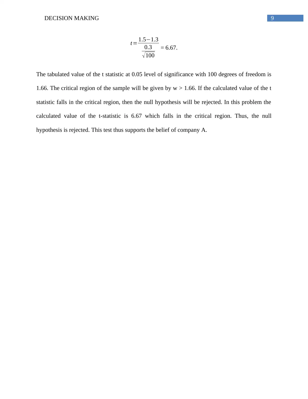
the sample size. Therefore, the value of the test statistic is

9DECISION MAKING
t= 1.5−1.3
0.3
√ 100
= 6.67.
The tabulated value of the t statistic at 0.05 level of significance with 100 degrees of freedom is
1.66. The critical region of the sample will be given by w > 1.66. If the calculated value of the t
statistic falls in the critical region, then the null hypothesis will be rejected. In this problem the
calculated value of the t-statistic is 6.67 which falls in the critical region. Thus, the null
hypothesis is rejected. This test thus supports the belief of company A.

10DECISION MAKING
REFERENCES
3101.0 - Australian Demographic Statistics, Sep 2016. (2017). Abs.gov.au. Retrieved 9 August
2017, from http://www.abs.gov.au/AUSSTATS/abs@.nsf/DetailsPage/3101.0Sep
%202016?OpenDocument
De Finetti, B. (2017). Theory of probability: A critical introductory treatment(Vol. 6). John
Wiley & Sons.
Miah, A. Q. (2016). Statistical Quality Control. In Applied Statistics for Social and Management
Sciences (pp. 353-384). Springer Singapore.
Miller, I., & Miller, M. (2015). John E. Freund's mathematical statistics with applications.
Pearson.