Classification Methods in Machine Learning

This article discusses the importance of classification methods in machine learning and their role in boosting data mining and performance analysis. It also explores how classification methods are used to determine true disabled persons. Additionally, it covers environment-driven and application-driven approaches in machine learning algorithms.

Section A
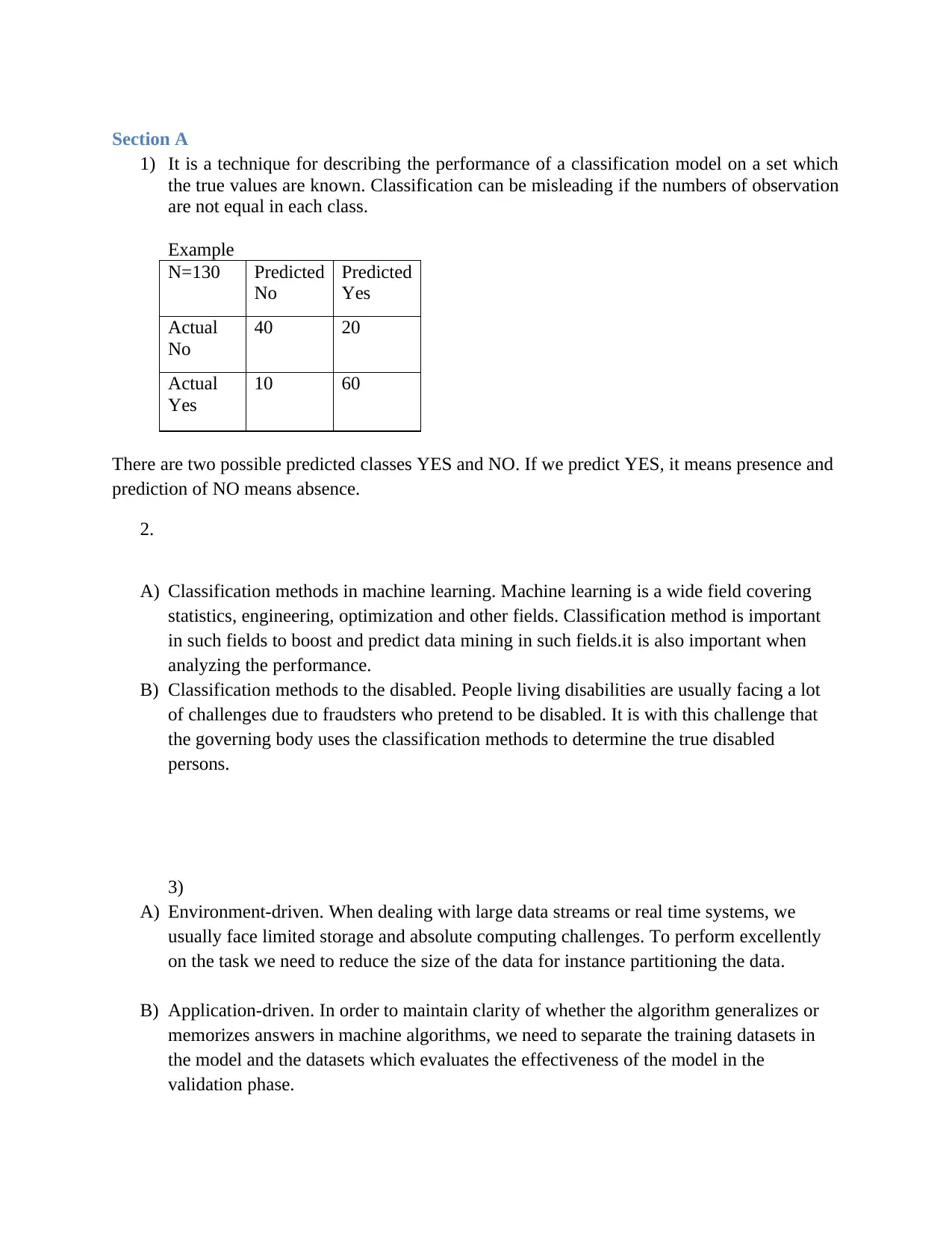
1) It is a technique for describing the performance of a classification model on a set which
the true values are known. Classification can be misleading if the numbers of observation
are not equal in each class.
Example
N=130 Predicted
No
Predicted
Yes
Actual
No
40 20
Actual
Yes
10 60
There are two possible predicted classes YES and NO. If we predict YES, it means presence and
prediction of NO means absence.
2.
A) Classification methods in machine learning. Machine learning is a wide field covering
statistics, engineering, optimization and other fields. Classification method is important
in such fields to boost and predict data mining in such fields.it is also important when
analyzing the performance.
B) Classification methods to the disabled. People living disabilities are usually facing a lot
of challenges due to fraudsters who pretend to be disabled. It is with this challenge that
the governing body uses the classification methods to determine the true disabled
persons.
3)
A) Environment-driven. When dealing with large data streams or real time systems, we
usually face limited storage and absolute computing challenges. To perform excellently
on the task we need to reduce the size of the data for instance partitioning the data.
B) Application-driven. In order to maintain clarity of whether the algorithm generalizes or
memorizes answers in machine algorithms, we need to separate the training datasets in
the model and the datasets which evaluates the effectiveness of the model in the
validation phase.

4)
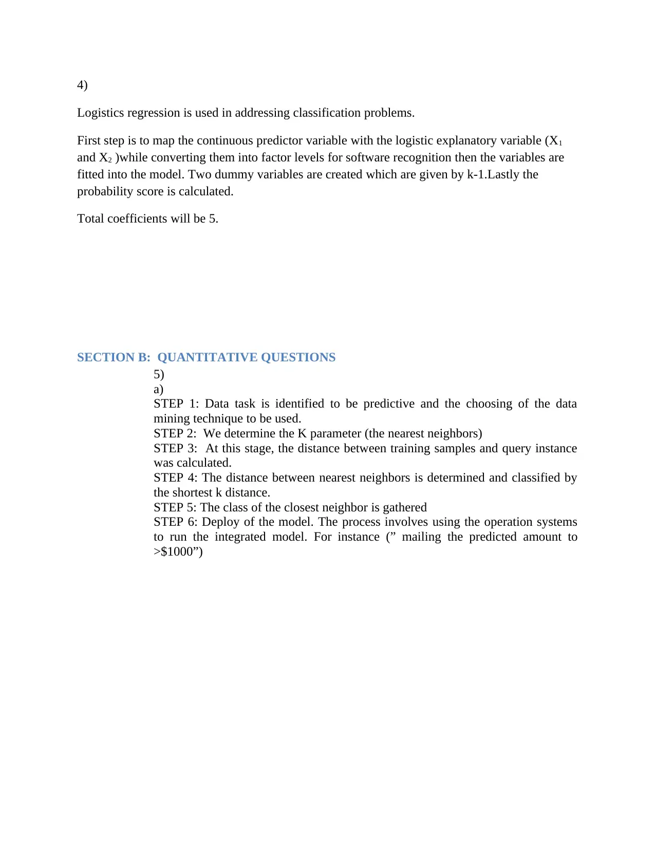
Logistics regression is used in addressing classification problems.
First step is to map the continuous predictor variable with the logistic explanatory variable (X1
and X2 )while converting them into factor levels for software recognition then the variables are
fitted into the model. Two dummy variables are created which are given by k-1.Lastly the
probability score is calculated.
Total coefficients will be 5.
SECTION B: QUANTITATIVE QUESTIONS
5)
a)
STEP 1: Data task is identified to be predictive and the choosing of the data
mining technique to be used.
STEP 2: We determine the K parameter (the nearest neighbors)
STEP 3: At this stage, the distance between training samples and query instance
was calculated.
STEP 4: The distance between nearest neighbors is determined and classified by
the shortest k distance.
STEP 5: The class of the closest neighbor is gathered
STEP 6: Deploy of the model. The process involves using the operation systems
to run the integrated model. For instance (” mailing the predicted amount to
>$1000”)

b)
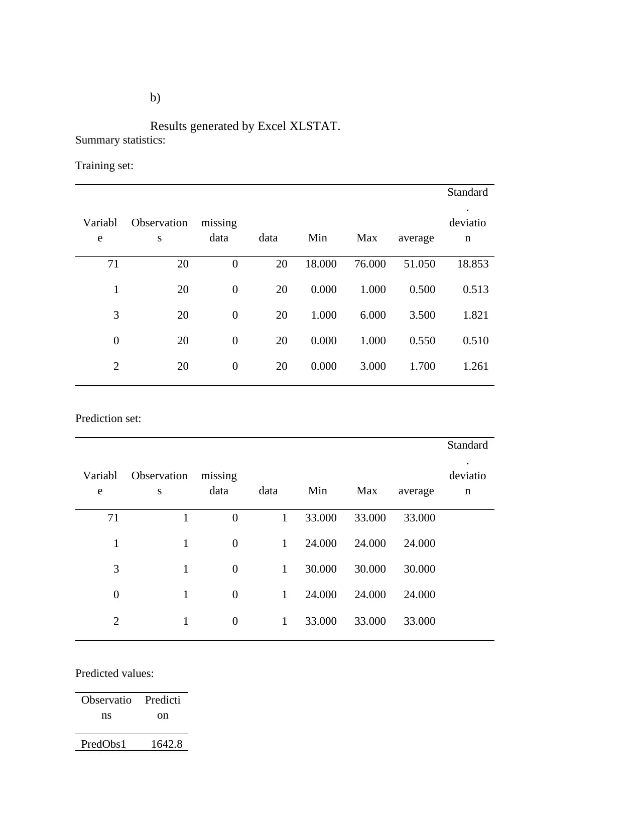
Results generated by Excel XLSTAT.
Summary statistics:
Training set:
Variabl
e
Observation
s
missing
data data Min Max average
Standard
.
deviatio
n
71 20 0 20 18.000 76.000 51.050 18.853
1 20 0 20 0.000 1.000 0.500 0.513
3 20 0 20 1.000 6.000 3.500 1.821
0 20 0 20 0.000 1.000 0.550 0.510
2 20 0 20 0.000 3.000 1.700 1.261
Prediction set:
Variabl
e
Observation
s
missing
data data Min Max average
Standard
.
deviatio
n
71 1 0 1 33.000 33.000 33.000
1 1 0 1 24.000 24.000 24.000
3 1 0 1 30.000 30.000 30.000
0 1 0 1 24.000 24.000 24.000
2 1 0 1 33.000 33.000 33.000
Predicted values:
Observatio
ns
Predicti
on
PredObs1 1642.8

Predicted spending’s by the 28 years old new female will be $1,642.8.
Question 6
Part a
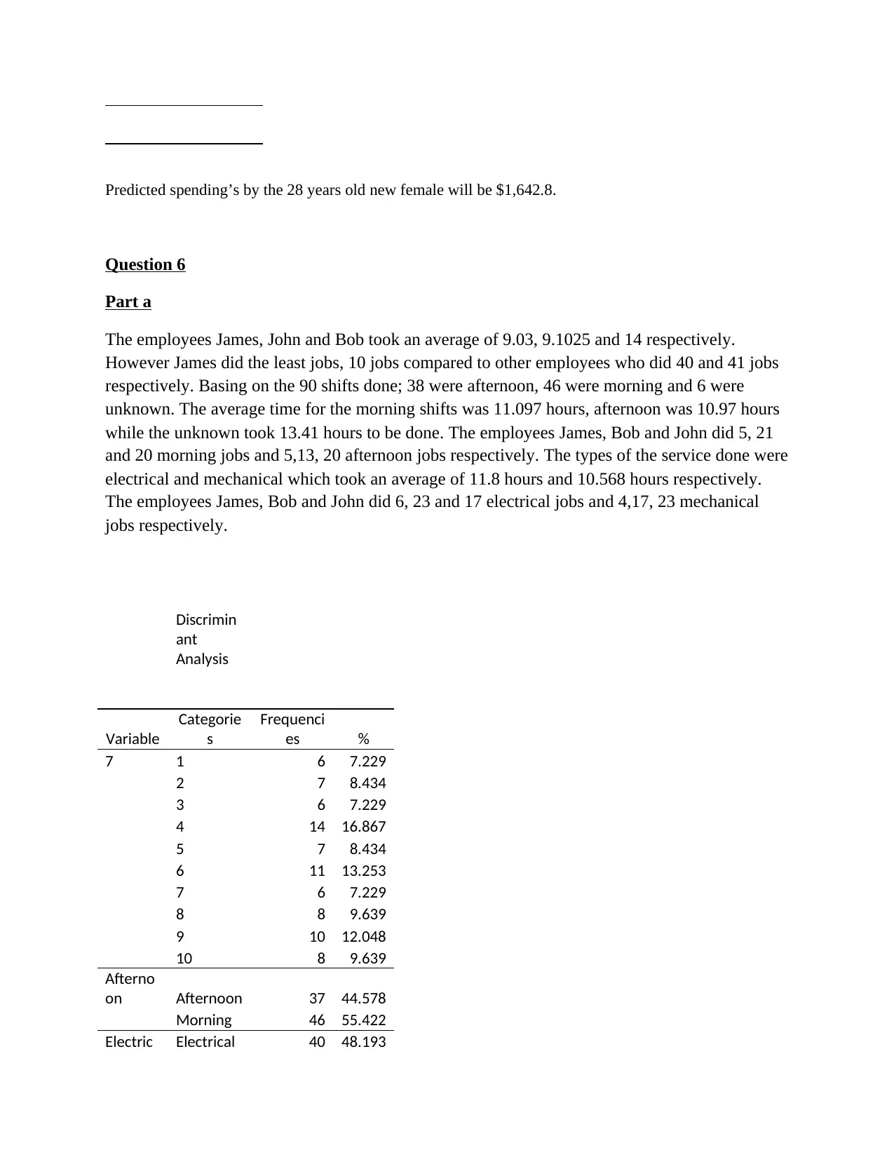
The employees James, John and Bob took an average of 9.03, 9.1025 and 14 respectively.
However James did the least jobs, 10 jobs compared to other employees who did 40 and 41 jobs
respectively. Basing on the 90 shifts done; 38 were afternoon, 46 were morning and 6 were
unknown. The average time for the morning shifts was 11.097 hours, afternoon was 10.97 hours
while the unknown took 13.41 hours to be done. The employees James, Bob and John did 5, 21
and 20 morning jobs and 5,13, 20 afternoon jobs respectively. The types of the service done were
electrical and mechanical which took an average of 11.8 hours and 10.568 hours respectively.
The employees James, Bob and John did 6, 23 and 17 electrical jobs and 4,17, 23 mechanical
jobs respectively.
Discrimin
ant
Analysis
Variable
Categorie
s
Frequenci
es %
7 1 6 7.229
2 7 8.434
3 6 7.229
4 14 16.867
5 7 8.434
6 11 13.253
7 6 7.229
8 8 9.639
9 10 12.048
10 8 9.639
Afterno
on Afternoon 37 44.578
Morning 46 55.422
Electric Electrical 40 48.193

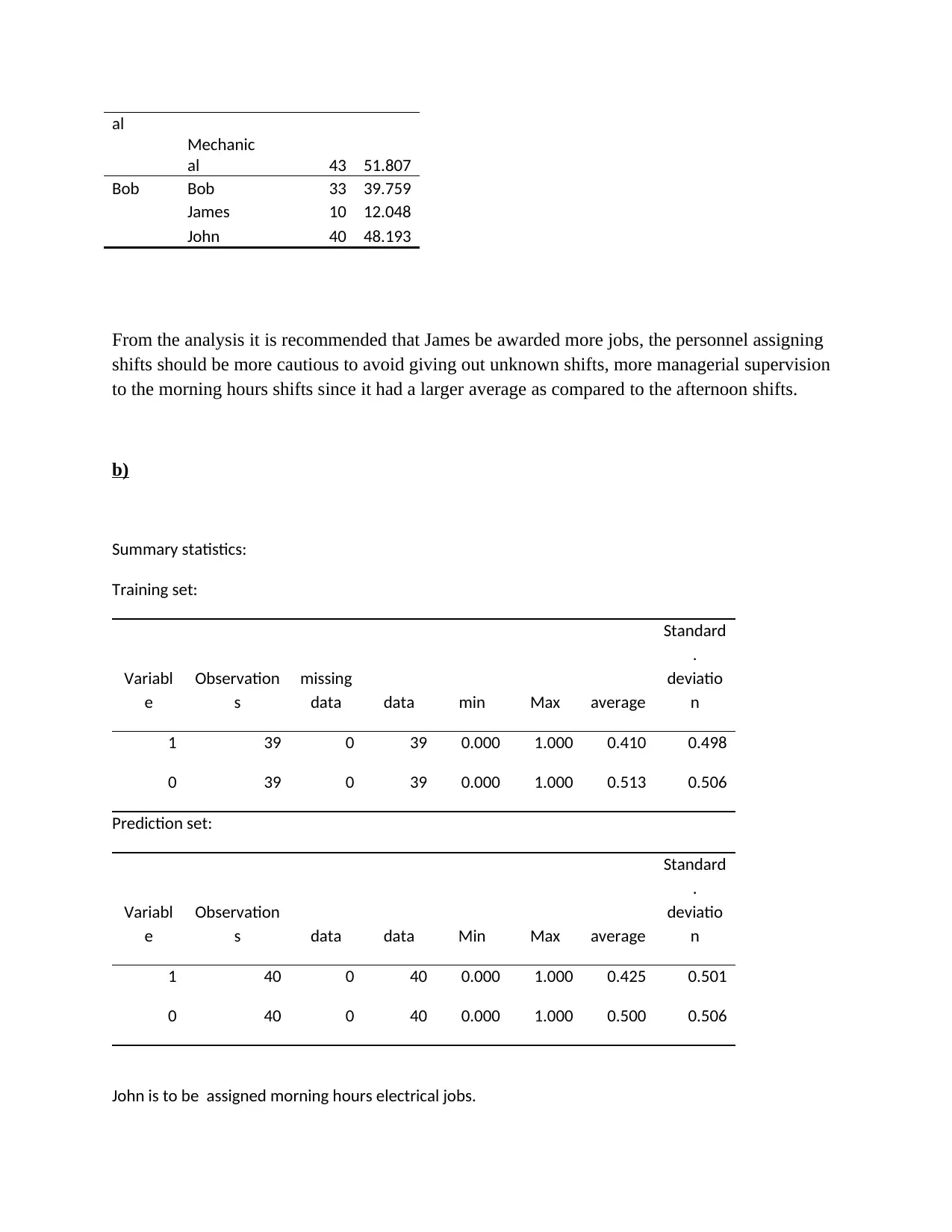
al
Mechanic
al 43 51.807
Bob Bob 33 39.759
James 10 12.048
John 40 48.193
From the analysis it is recommended that James be awarded more jobs, the personnel assigning
shifts should be more cautious to avoid giving out unknown shifts, more managerial supervision
to the morning hours shifts since it had a larger average as compared to the afternoon shifts.
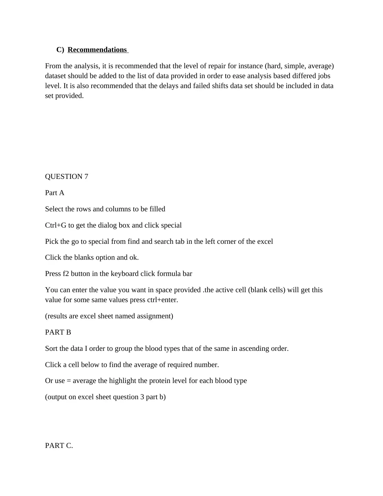
b)
Summary statistics:
Training set:
Variabl
e
Observation
s
missing
data data min Max average
Standard
.
deviatio
n
1 39 0 39 0.000 1.000 0.410 0.498
0 39 0 39 0.000 1.000 0.513 0.506
Prediction set:
Variabl
e
Observation
s data data Min Max average
Standard
.
deviatio
n
1 40 0 40 0.000 1.000 0.425 0.501
0 40 0 40 0.000 1.000 0.500 0.506
John is to be assigned morning hours electrical jobs.

C) Recommendations
From the analysis, it is recommended that the level of repair for instance (hard, simple, average)
dataset should be added to the list of data provided in order to ease analysis based differed jobs
level. It is also recommended that the delays and failed shifts data set should be included in data
set provided.
QUESTION 7
Part A
Select the rows and columns to be filled
Ctrl+G to get the dialog box and click special
Pick the go to special from find and search tab in the left corner of the excel
Click the blanks option and ok.
Press f2 button in the keyboard click formula bar
You can enter the value you want in space provided .the active cell (blank cells) will get this
value for some same values press ctrl+enter.
(results are excel sheet named assignment)
PART B
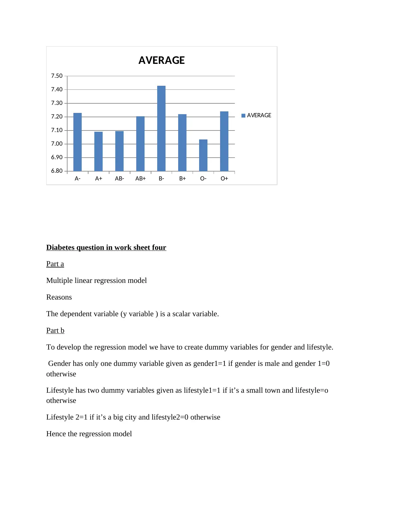
Sort the data I order to group the blood types that of the same in ascending order.
Click a cell below to find the average of required number.
Or use = average the highlight the protein level for each blood type
(output on excel sheet question 3 part b)
PART C.

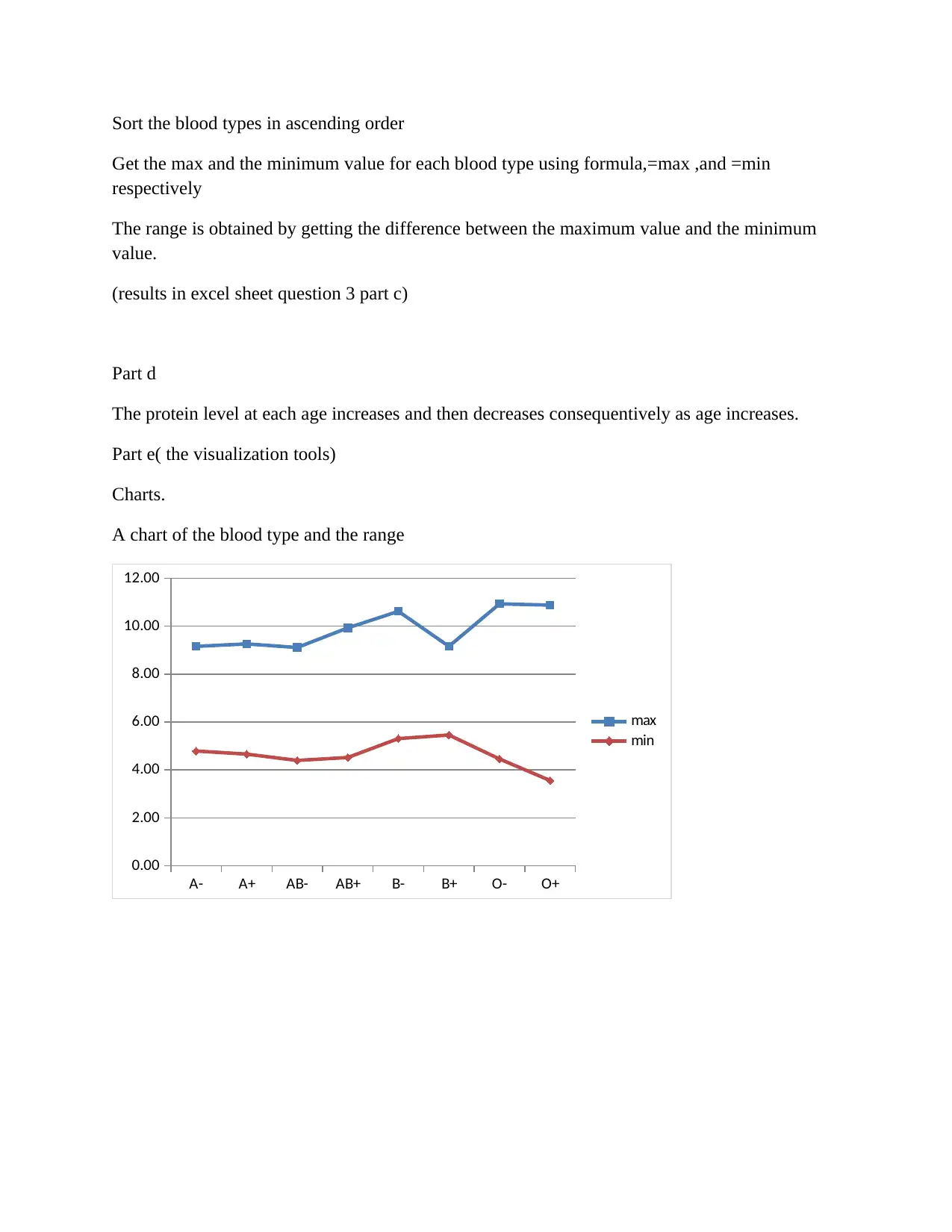
Sort the blood types in ascending order
Get the max and the minimum value for each blood type using formula,=max ,and =min
respectively
The range is obtained by getting the difference between the maximum value and the minimum
value.
(results in excel sheet question 3 part c)
Part d
The protein level at each age increases and then decreases consequentively as age increases.
Part e( the visualization tools)
Charts.
A chart of the blood type and the range
A- A+ AB- AB+ B- B+ O- O+
0.00
2.00
4.00
6.00
8.00
10.00
12.00
max
min

A- A+ AB- AB+ B- B+ O- O+
6.80
6.90
7.00
7.10
7.20
7.30
7.40
7.50
AVERAGE
AVERAGE
Diabetes question in work sheet four
Part a
Multiple linear regression model
Reasons
The dependent variable (y variable ) is a scalar variable.
Part b
To develop the regression model we have to create dummy variables for gender and lifestyle.
Gender has only one dummy variable given as gender1=1 if gender is male and gender 1=0
otherwise
Lifestyle has two dummy variables given as lifestyle1=1 if it’s a small town and lifestyle=o
otherwise
Lifestyle 2=1 if it’s a big city and lifestyle2=0 otherwise
Hence the regression model

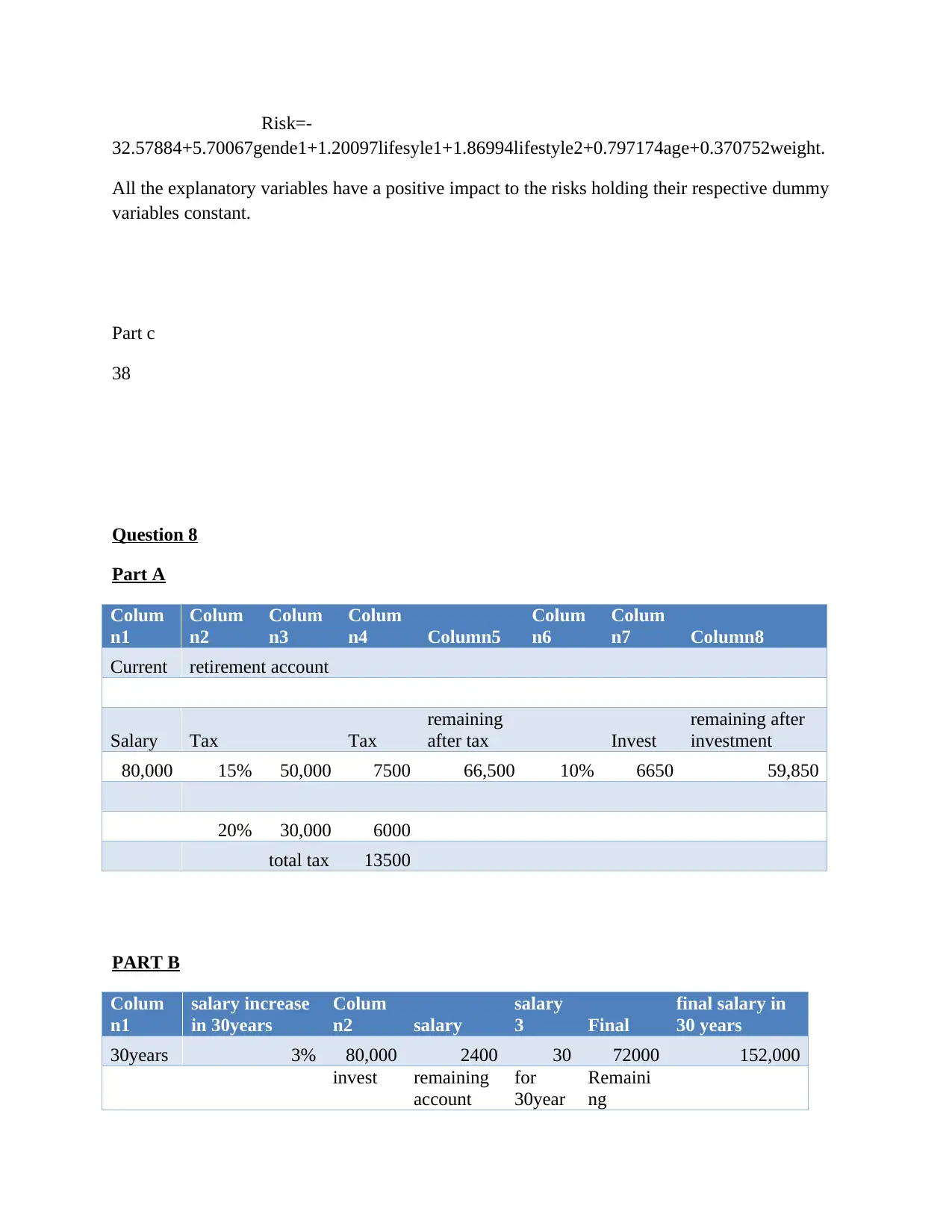
Risk=-
32.57884+5.70067gende1+1.20097lifesyle1+1.86994lifestyle2+0.797174age+0.370752weight.
All the explanatory variables have a positive impact to the risks holding their respective dummy
variables constant.
Part c
38
Question 8
Part A
Colum
n1
Colum
n2
Colum
n3
Colum
n4 Column5
Colum
n6
Colum
n7 Column8
Current retirement account
Salary Tax Tax
remaining
after tax Invest
remaining after
investment
80,000 15% 50,000 7500 66,500 10% 6650 59,850
20% 30,000 6000
total tax 13500
PART B
Colum
n1
salary increase
in 30years
Colum
n2 salary
salary
3 Final
final salary in
30 years
30years 3% 80,000 2400 30 72000 152,000
invest remaining
account
for
30year
Remaini
ng

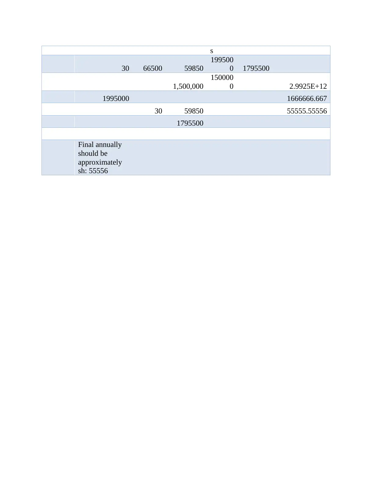
s
30 66500 59850
199500
0 1795500
1,500,000
150000
0 2.9925E+12
1995000 1666666.667
30 59850 55555.55556
1795500
Final annually
should be
approximately
sh: 55556