Selected Statistical Problems with ANOVA and Regression Analysis

This article presents selected statistical problems with ANOVA and regression analysis. It includes frequency distribution table, histogram, ANOVA table, regression table, hypothesis testing, and interpretation of results.

1
Selected Statistical Problems
Student Name: Student ID:
Unit Name: Unit ID:
Date Due: Professor Name:

2
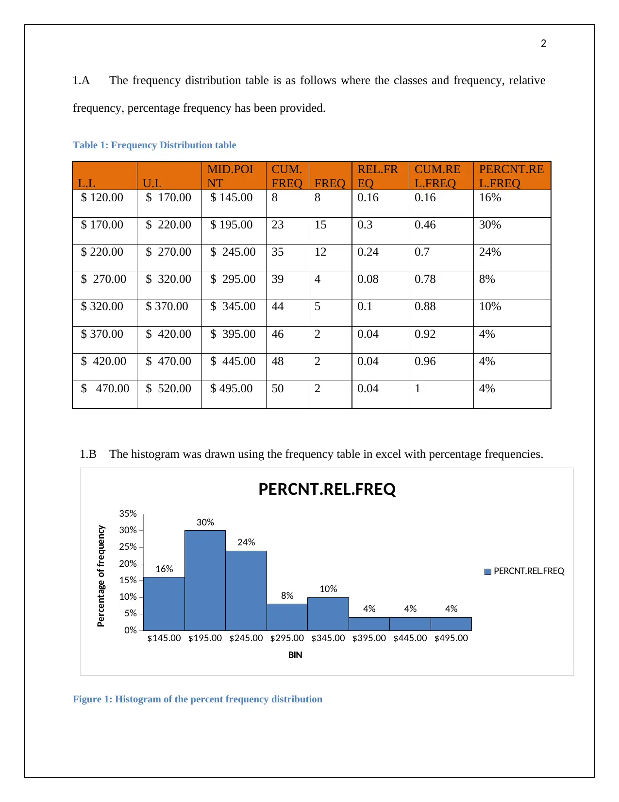
1.A The frequency distribution table is as follows where the classes and frequency, relative
frequency, percentage frequency has been provided.
Table 1: Frequency Distribution table
L.L U.L
MID.POI
NT
CUM.
FREQ FREQ
REL.FR
EQ
CUM.RE
L.FREQ
PERCNT.RE
L.FREQ
$ 120.00 $ 170.00 $ 145.00 8 8 0.16 0.16 16%
$ 170.00 $ 220.00 $ 195.00 23 15 0.3 0.46 30%
$ 220.00 $ 270.00 $ 245.00 35 12 0.24 0.7 24%
$ 270.00 $ 320.00 $ 295.00 39 4 0.08 0.78 8%
$ 320.00 $ 370.00 $ 345.00 44 5 0.1 0.88 10%
$ 370.00 $ 420.00 $ 395.00 46 2 0.04 0.92 4%
$ 420.00 $ 470.00 $ 445.00 48 2 0.04 0.96 4%
$ 470.00 $ 520.00 $ 495.00 50 2 0.04 1 4%
1.B The histogram was drawn using the frequency table in excel with percentage frequencies.
$145.00 $195.00 $245.00 $295.00 $345.00 $395.00 $445.00 $495.00
0%
5%
10%
15%
20%
25%
30%
35%
16%
30%
24%
8% 10%
4% 4% 4%
PERCNT.REL.FREQ
PERCNT.REL.FREQ
BIN
Percentage of frequency
Figure 1: Histogram of the percent frequency distribution

3
1.C The histogram was right skewed in nature, which was indicative of the not normal nature
of the data set of Missy Walters’ assistant. Hence, Median was the best choice of central
tendency or measure of location. The Mean would have been also a good choice as measure but
Median was the appropriate selection as measure of location.
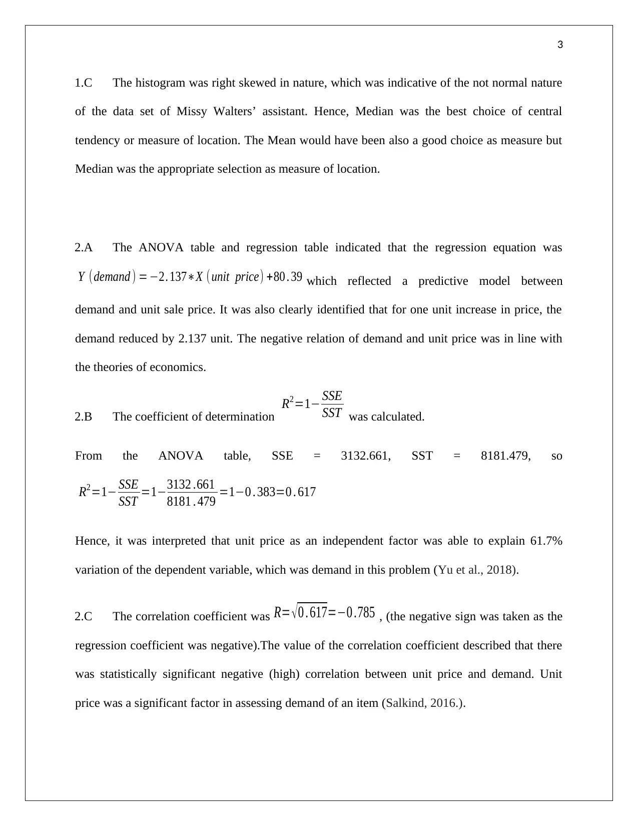
2.A The ANOVA table and regression table indicated that the regression equation was
Y (demand ) = −2. 137∗X ( unit price) +80 . 39 which reflected a predictive model between
demand and unit sale price. It was also clearly identified that for one unit increase in price, the
demand reduced by 2.137 unit. The negative relation of demand and unit price was in line with
the theories of economics.
2.B The coefficient of determination
R2=1− SSE
SST was calculated.
From the ANOVA table, SSE = 3132.661, SST = 8181.479, so
R2=1− SSE
SST =1−3132 .661
8181 . 479 =1−0 . 383=0 . 617
Hence, it was interpreted that unit price as an independent factor was able to explain 61.7%
variation of the dependent variable, which was demand in this problem (Yu et al., 2018).
2.C The correlation coefficient was R= √ 0 . 617=−0 .785 , (the negative sign was taken as the
regression coefficient was negative).The value of the correlation coefficient described that there
was statistically significant negative (high) correlation between unit price and demand. Unit
price was a significant factor in assessing demand of an item (Salkind, 2016.).

4
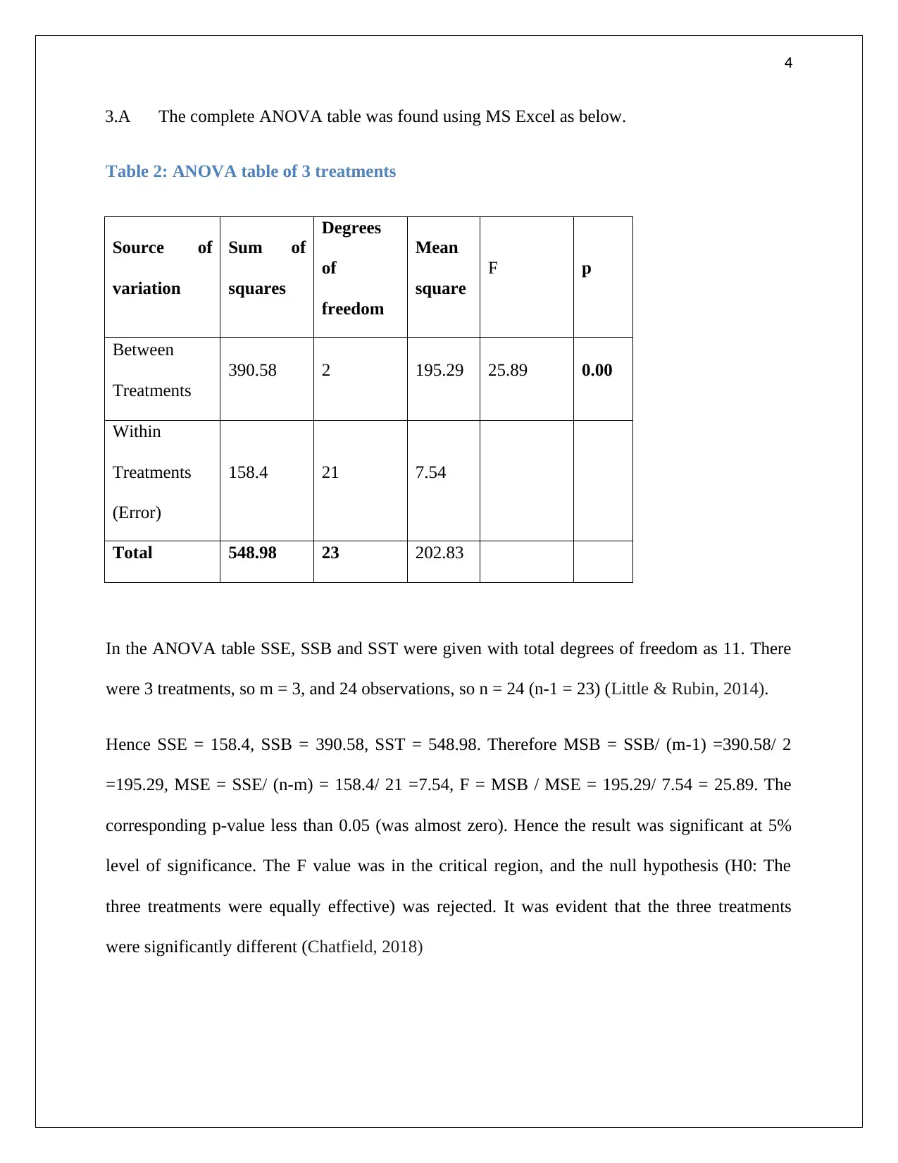
3.A The complete ANOVA table was found using MS Excel as below.
Table 2: ANOVA table of 3 treatments
Source of
variation
Sum of
squares
Degrees
of
freedom
Mean
square
F p
Between
Treatments
390.58 2 195.29 25.89 0.00
Within
Treatments
(Error)
158.4 21 7.54
Total 548.98 23 202.83
In the ANOVA table SSE, SSB and SST were given with total degrees of freedom as 11. There
were 3 treatments, so m = 3, and 24 observations, so n = 24 (n-1 = 23) (Little & Rubin, 2014).
Hence SSE = 158.4, SSB = 390.58, SST = 548.98. Therefore MSB = SSB/ (m-1) =390.58/ 2
=195.29, MSE = SSE/ (n-m) = 158.4/ 21 =7.54, F = MSB / MSE = 195.29/ 7.54 = 25.89. The
corresponding p-value less than 0.05 (was almost zero). Hence the result was significant at 5%
level of significance. The F value was in the critical region, and the null hypothesis (H0: The
three treatments were equally effective) was rejected. It was evident that the three treatments
were significantly different (Chatfield, 2018)

5
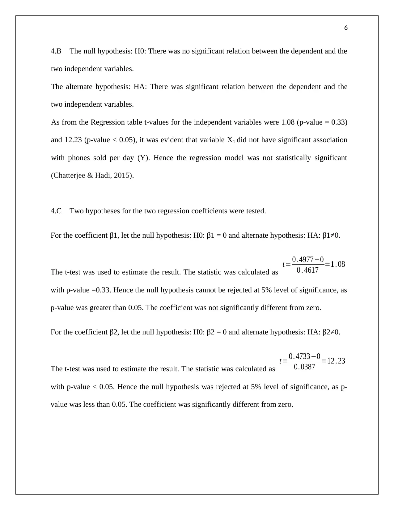
4.A The complete table of the problem was found using MS Excel as follows.
Table 3: Complete ANOVA and Regression Table
ANOVA
Df SS MS f p
Regressio
n 2 40.7 20.35 80.1181102 0.000593
Residual 4 1.016 0.254
Total 6 41.716 20.604
Regression Table
Coefficients Standard Error t p
Intercept 0.8051 0.0698 11.54 0.00
X1 0.4977 0.4617 1.08 0.33
X2 0.4733 0.0387 12.23 0.00
The above table was completed following the calculations below:
N = 7, so total degree of freedom = N – 1 = 6. There were two independent variables, so DF for
regression was 2, for residual it was (6 – 2 = 4). Now SSB = 40.7 and SSE = 1.016, so SST =
(40.7 + 1.016) = 41.716. MSB = SSB /2 = 20.35, MSE = SSE/ 4 = 0.254. MST = MSB + MSE. F
value was the ratio between MSB and MSE. P-value was calculated from the F-distribution
function in excel (Glantz, Slinker & Neilands, 2016).
In regression table standard error of intercept was found as
SEslope= √ SSE /( n−2 )
√ SST and t-values
were the ratio of coefficients and standard errors. The p-values were found using the t-
distribution function in excel.
From the regression table, the estimated regression model was
Y =0 . 8051+0 . 4977 X1+ 0. 4733 X2

6
4.B The null hypothesis: H0: There was no significant relation between the dependent and the
two independent variables.
The alternate hypothesis: HA: There was significant relation between the dependent and the
two independent variables.
As from the Regression table t-values for the independent variables were 1.08 (p-value = 0.33)
and 12.23 (p-value < 0.05), it was evident that variable X1 did not have significant association
with phones sold per day (Y). Hence the regression model was not statistically significant
(Chatterjee & Hadi, 2015).
4.C Two hypotheses for the two regression coefficients were tested.
For the coefficient β1, let the null hypothesis: H0: β1 = 0 and alternate hypothesis: HA: β1≠0.
The t-test was used to estimate the result. The statistic was calculated as
t = 0. 4977−0
0 . 4617 =1 . 08
with p-value =0.33. Hence the null hypothesis cannot be rejected at 5% level of significance, as
p-value was greater than 0.05. The coefficient was not significantly different from zero.
For the coefficient β2, let the null hypothesis: H0: β2 = 0 and alternate hypothesis: HA: β2≠0.
The t-test was used to estimate the result. The statistic was calculated as
t = 0. 4733−0
0. 0387 =12 . 23
with p-value < 0.05. Hence the null hypothesis was rejected at 5% level of significance, as p-
value was less than 0.05. The coefficient was significantly different from zero.

7
4.D The slope was 0.8051 for the regression equation and noticeable fact was that the
coefficient was positive with p- value < 0.05. Hence it was interpreted that mobiles sold per day
had a significant sales figure when the independent factors were zero.
4.E From the regression equation Y =0 . 8051+0 . 4977 X1+ 0. 4733 X2 , taking X1= $20,000
and X2 = 10, Y =0 . 8051+0 . 4977∗20000+0 . 4733∗10=9959 . 5≃9960
Therefore, predicted sales of phones was 9960 (units) (Balint, 2018).
References
Balint, M., 2018. Thrills and regressions. Routledge.
Chatfield, C., 2018. Statistics for technology: a course in applied statistics. Routledge.
Chatterjee, S. and Hadi, A.S., 2015. Regression analysis by example. John Wiley & Sons.
Glantz, S.A., Slinker, B.K. and Neilands, T.B., 2016. Primer of applied regression & analysis of
variance. McGraw-Hill Medical Publishing Division.
Little, R.J. and Rubin, D.B., 2014. Statistical analysis with missing data (Vol. 333). John Wiley
& Sons.
Little, R.J. and Rubin, D.B., 2014. Statistical analysis with missing data (Vol. 333). John Wiley
& Sons.
Salkind, N.J., 2016. Statistics for people who (think they) hate statistics. Sage Publications.

8
Yu, G., Zhu, L., Sun, J. and Robison, L.L., 2018. Regression analysis of incomplete data from
event history studies with the proportional rates model. Statistics and its interface, 11(1), p.91.