SPSS Data Analysis: Pearson’s Correlation, Chi-square and Two-way ANOVA Testing

This article explains the SPSS data analysis of Pearson’s Correlation, Chi-square and Two-way ANOVA Testing. It includes hypothesis, interpretation and conclusion of each test. The summary of the analysis is also provided.

1

2
Table of Contents
Part A: Pearson’s Correlation Analysis:..........................................................................................2
A. a) Hypothesis of Correlation test:...........................................................................................2
A. b) Interpretation and Conclusion of Correlation test:.............................................................3
Part B: Chi-square testing:...............................................................................................................4
B. a) Hypothesis of Chi-square test:............................................................................................4
B. b) Interpretation and Conclusion of Chi-square test:..............................................................5
Part C. Two-way ANOVA testing:..................................................................................................6
C. a) Hypothesis of Two-way ANOVA test:...............................................................................6
C. b) Interpretation and Conclusion of Two-way ANOVA test:.................................................7
Summary of the Analysis:...............................................................................................................8
Table of Figures
Table 1: Pearson Correlation co-efficient matrix............................................................................3
Table 2: Cross tabulation.................................................................................................................5
Table 3: Chi-square test to find association or significance............................................................5
Table 4: Descriptive statistics of Two-way ANOVA test...............................................................7
Table 5: Tests of between-subjects effect of Two-way ANOVA test.............................................7

3
Part A: Pearson’s Correlation Analysis:
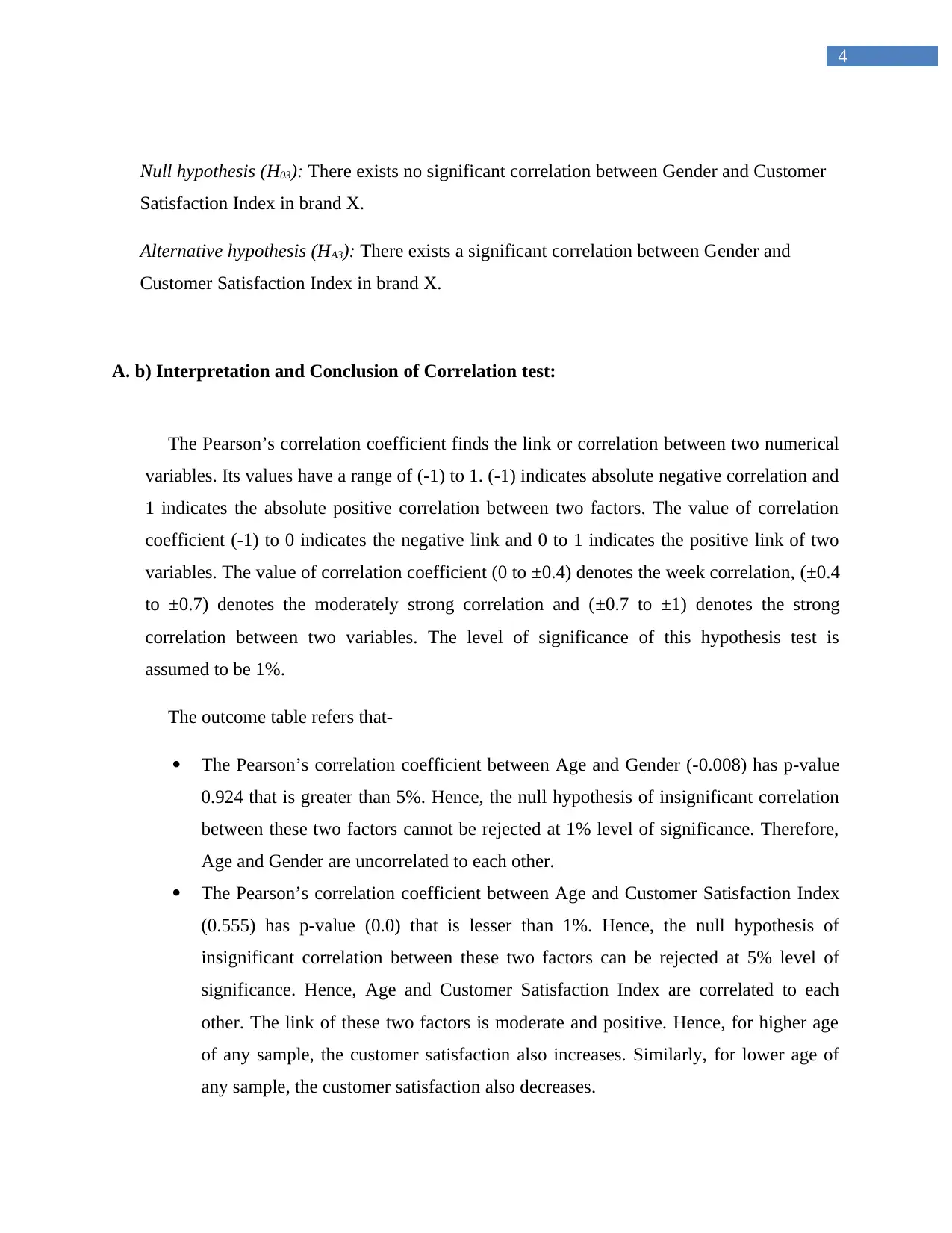
Table 1: Pearson Correlation co-efficient matrix
A. a) Hypothesis of Correlation test:
The hypotheses are-
Null hypothesis (H01): There exists no significant correlation between Age and Gender.
Alternative hypothesis (HA1): There exists a significant correlation between Age and Gender.
Null hypothesis (H02): There exists no significant correlation between Age and Customer
Satisfaction Index in brand X.
Alternative hypothesis (HA2): There exists a significant correlation between Age and
Customer Satisfaction Index in brand X.

4
Null hypothesis (H03): There exists no significant correlation between Gender and Customer
Satisfaction Index in brand X.
Alternative hypothesis (HA3): There exists a significant correlation between Gender and
Customer Satisfaction Index in brand X.
A. b) Interpretation and Conclusion of Correlation test:
The Pearson’s correlation coefficient finds the link or correlation between two numerical
variables. Its values have a range of (-1) to 1. (-1) indicates absolute negative correlation and
1 indicates the absolute positive correlation between two factors. The value of correlation
coefficient (-1) to 0 indicates the negative link and 0 to 1 indicates the positive link of two
variables. The value of correlation coefficient (0 to ±0.4) denotes the week correlation, (±0.4
to ±0.7) denotes the moderately strong correlation and (±0.7 to ±1) denotes the strong
correlation between two variables. The level of significance of this hypothesis test is
assumed to be 1%.
The outcome table refers that-
 The Pearson’s correlation coefficient between Age and Gender (-0.008) has p-value
0.924 that is greater than 5%. Hence, the null hypothesis of insignificant correlation
between these two factors cannot be rejected at 1% level of significance. Therefore,
Age and Gender are uncorrelated to each other.
 The Pearson’s correlation coefficient between Age and Customer Satisfaction Index
(0.555) has p-value (0.0) that is lesser than 1%. Hence, the null hypothesis of
insignificant correlation between these two factors can be rejected at 5% level of
significance. Hence, Age and Customer Satisfaction Index are correlated to each
other. The link of these two factors is moderate and positive. Hence, for higher age
of any sample, the customer satisfaction also increases. Similarly, for lower age of
any sample, the customer satisfaction also decreases.

5
 The Pearson’s correlation coefficient between Customer Satisfaction Index and
Gender (0.322) has p-value (0.0) that is less than 1%. Therefore, the null hypothesis
of insignificant correlation between these two factors can be rejected at 5% level of
significance. Hence, Gender and Customer Satisfaction Index are weekly but
significantly correlated to each other. It indicates that males (=1) are more satisfied
as per greater satisfaction index rather than females (=0).
Part B: Chi-square testing:
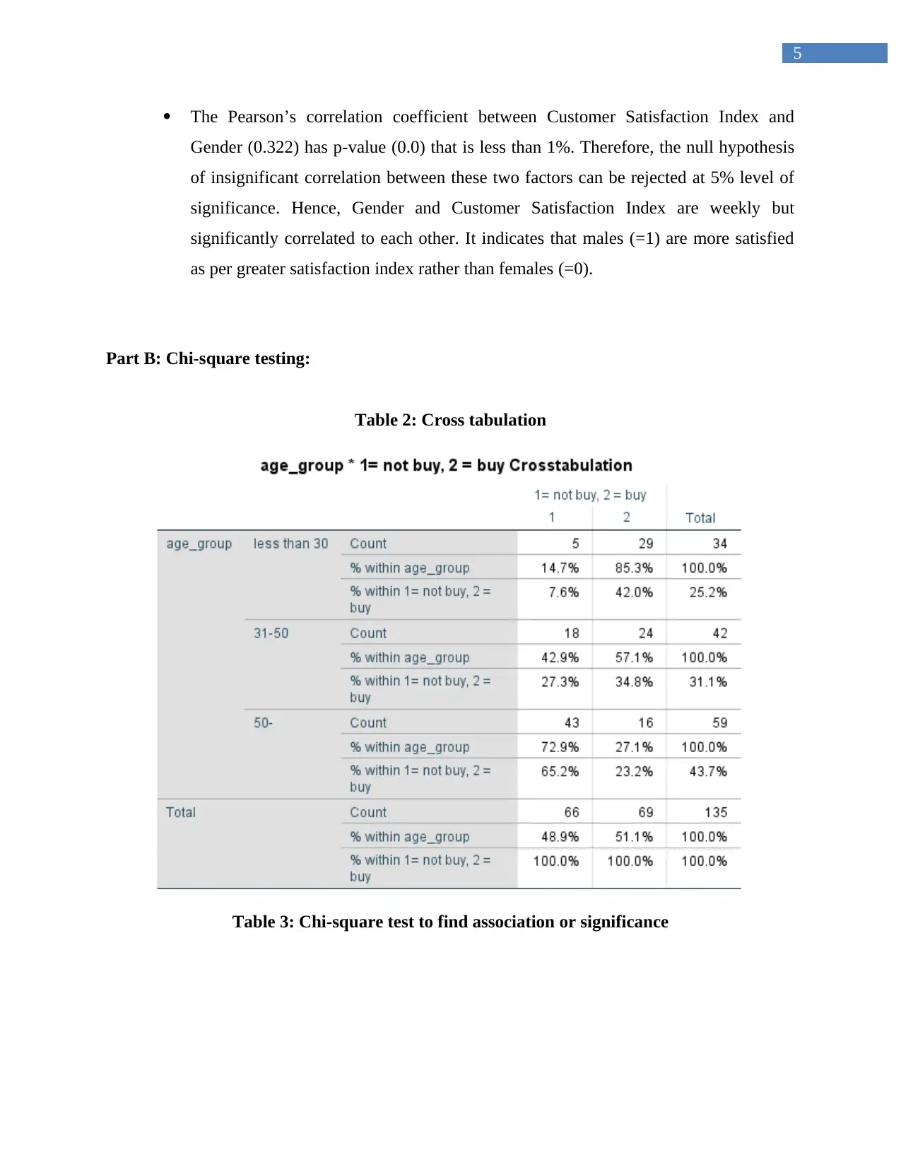
Table 2: Cross tabulation
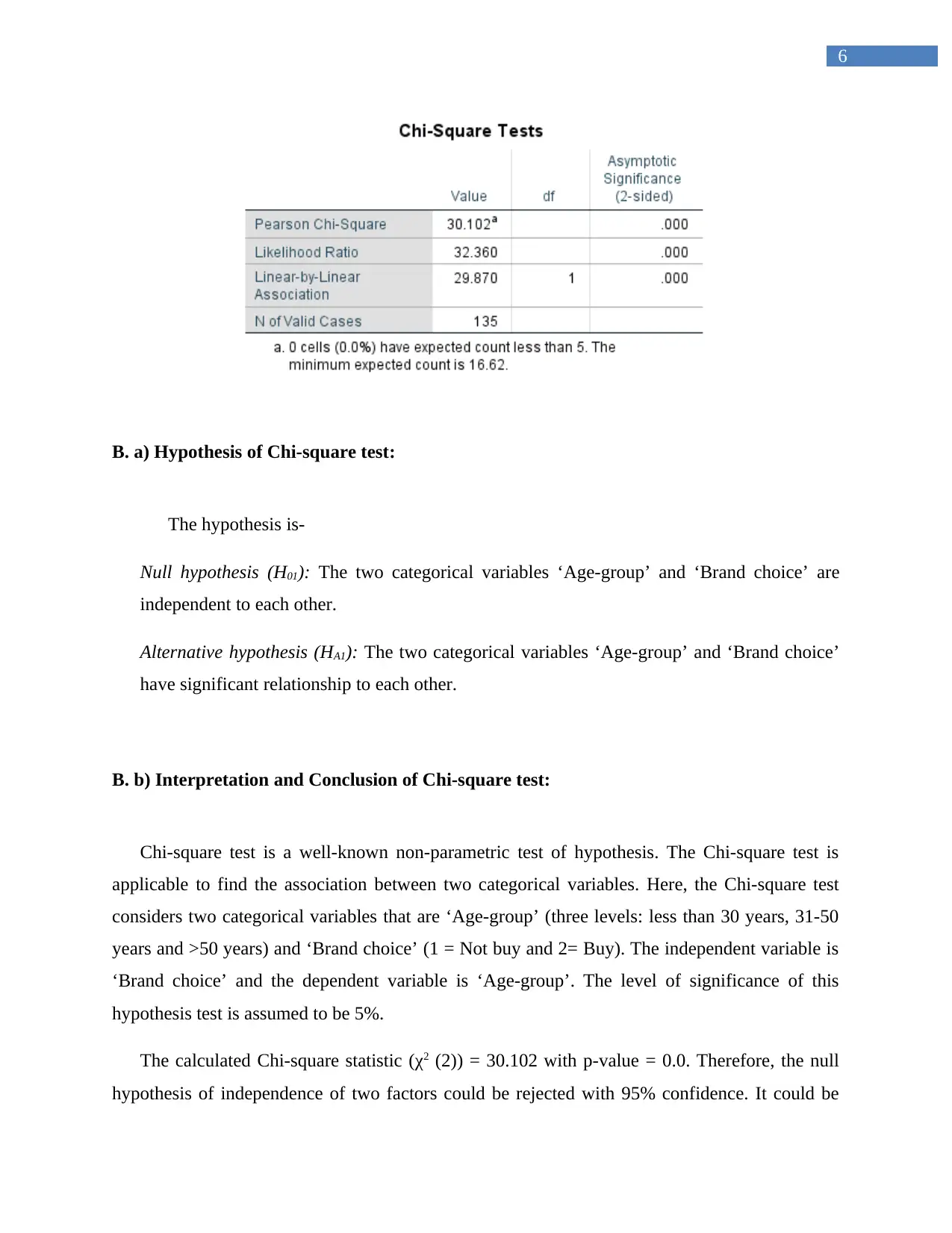
Table 3: Chi-square test to find association or significance

6
B. a) Hypothesis of Chi-square test:
The hypothesis is-
Null hypothesis (H01): The two categorical variables ‘Age-group’ and ‘Brand choice’ are
independent to each other.
Alternative hypothesis (HA1): The two categorical variables ‘Age-group’ and ‘Brand choice’
have significant relationship to each other.
B. b) Interpretation and Conclusion of Chi-square test:
Chi-square test is a well-known non-parametric test of hypothesis. The Chi-square test is
applicable to find the association between two categorical variables. Here, the Chi-square test
considers two categorical variables that are ‘Age-group’ (three levels: less than 30 years, 31-50
years and >50 years) and ‘Brand choice’ (1 = Not buy and 2= Buy). The independent variable is
‘Brand choice’ and the dependent variable is ‘Age-group’. The level of significance of this
hypothesis test is assumed to be 5%.
The calculated Chi-square statistic (χ2 (2)) = 30.102 with p-value = 0.0. Therefore, the null
hypothesis of independence of two factors could be rejected with 95% confidence. It could be

7
interpreted that different age-groups and various brand-choices are related to each other. These
two factors are not at all independent to each other. It further concludes that there exists
significant difference between observed and expected frequencies of the cross-tabulation table.
Part C. Two-way ANOVA testing:
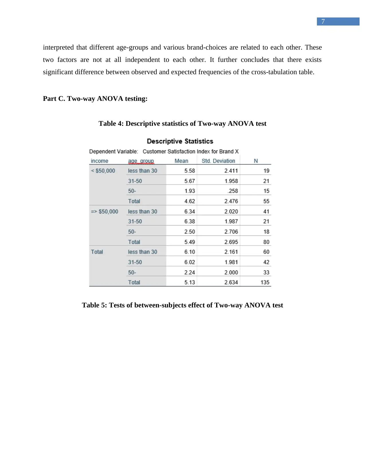
Table 4: Descriptive statistics of Two-way ANOVA test
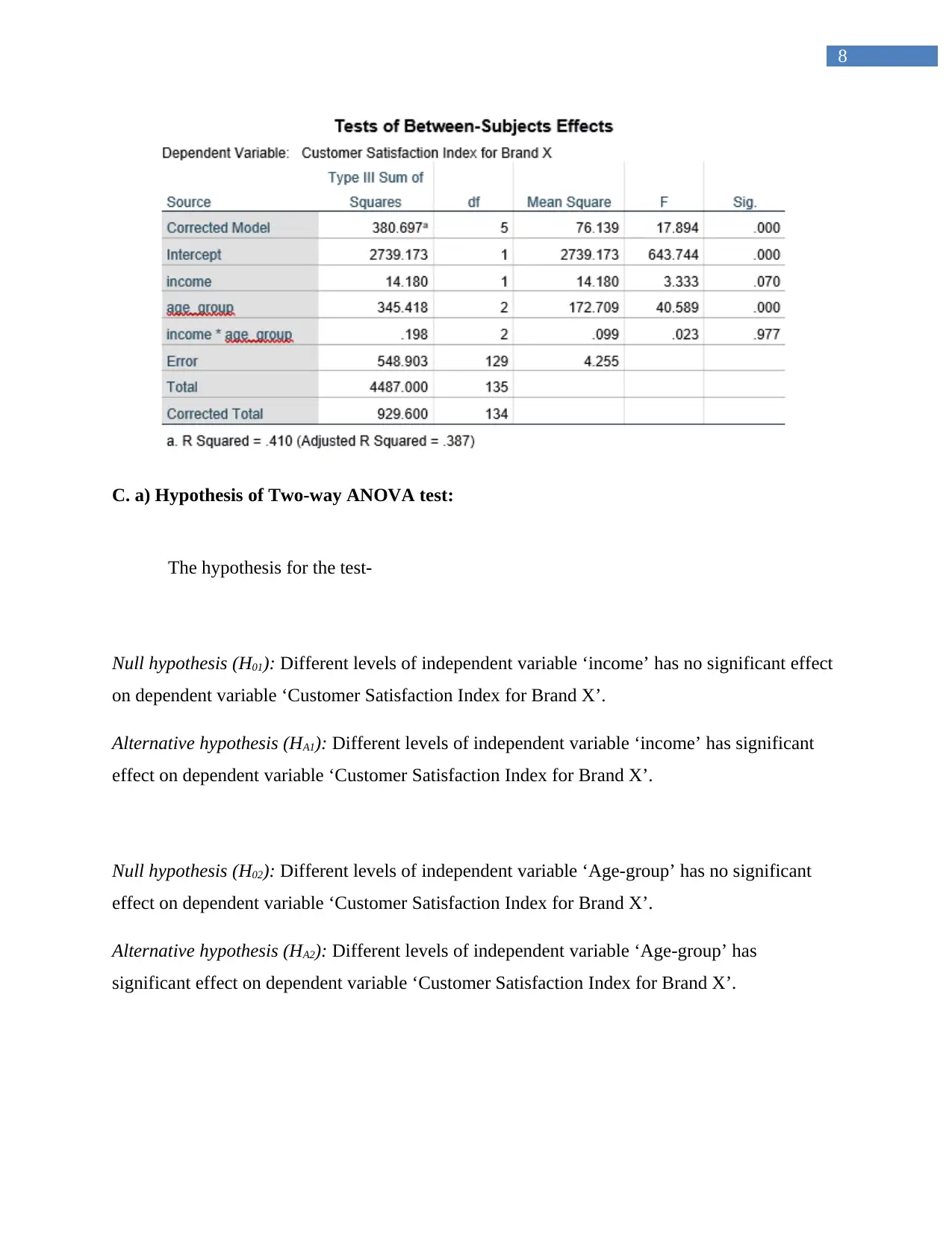
Table 5: Tests of between-subjects effect of Two-way ANOVA test

8
C. a) Hypothesis of Two-way ANOVA test:
The hypothesis for the test-
Null hypothesis (H01): Different levels of independent variable ‘income’ has no significant effect
on dependent variable ‘Customer Satisfaction Index for Brand X’.
Alternative hypothesis (HA1): Different levels of independent variable ‘income’ has significant
effect on dependent variable ‘Customer Satisfaction Index for Brand X’.
Null hypothesis (H02): Different levels of independent variable ‘Age-group’ has no significant
effect on dependent variable ‘Customer Satisfaction Index for Brand X’.
Alternative hypothesis (HA2): Different levels of independent variable ‘Age-group’ has
significant effect on dependent variable ‘Customer Satisfaction Index for Brand X’.

9
Null hypothesis (H03): For different levels of independent variable ‘Age-group’ with respect to
various ‘income’ levels, the values of dependent variable ‘Customer Satisfaction Index for Brand
X’ do not vary.
Alternative hypothesis (HA3): For different levels of independent variable ‘Age-group’ with
respect to various ‘income’ levels, the values of dependent variable ‘Customer Satisfaction Index
for Brand X’ vary.
C. b) Interpretation and Conclusion of Two-way ANOVA test:
The two-way ANOVA test is applied to test the hypotheses. The test investigates the equality
and variability of customer satisfaction index with respect to the independent variables and their
interaction effects. The dependent variable for this test is assumed to be ‘Customer Satisfaction
Index for Brand X’ and the independent variables for this test is assumed to be ‘Income’ and
‘Age-group’. The ‘Two-way ANOVA test’ includes the results of ‘descriptives’ and ‘between-
subjects effects’. The outcome tables interpret that-
 The F-statistic of main effect ‘Income’ is 3.333 (d.f = 1) with p-value 0.7. The p-values is
greater than 0.05. The null hypothesis could not be rejected with 95% confidence. Hence,
no difference of customer satisfaction index is observed for different income levels
(<$50,000 and ≥$50,000) when the effect of ‘Age-group’ is absent.
 The F-statistic of main effect ‘Age-group’ is 40.589 (d.f. = 2) with p-value 0.0. The p-
value is less than 0.05. The null hypothesis could be rejected with 95% confidence.
Therefore, difference of customer satisfaction index is observed for various age-groups
(less than 30 years, 31-50 years and more than 50 years) while the effect of ‘Income’ is
absent.
 The F-statistic of interaction effect of two main effects ‘Income’ and ‘Age-group’ is
0.023 (d.f. = 2) with p-value 0.977. The null hypothesis of insignificant effect of

10
‘Income’ and ‘Age-group’ could not be rejected with 95% probability. Hence, there
exists significant differences of customer satisfaction indexes between various levels of
‘Age-group’ with respect to different levels of ‘Income’. Note that, the effects of both the
independent variables are simultaneously present in this context.
Summary of the Analysis:
The SPSS data analysis summarizes that age and gender of the samples are not
significantly correlated. However, age and customer satisfaction index are positively and
significantly correlated to each other. Similarly, gender type and customer satisfaction index are
positively and significantly correlated. Also, it was found that brand choice (buying or not
buying) is dependent upon the age-group of the samples.
In the next stage it was discovered that variation in age-groups is a cause of variation in
customer satisfaction index for brand X. However, the variation in income levels is not a cause
of variation in customer satisfaction index for brand X. Further, the joint effect of age-groups
and income groups is not a significant cause of customer satisfaction index for brand X.
Overall it is found that age-groups are the significant predictors of customer satisfaction
index in brand X; however, gender and income categories cannot truly predict the variability of
customer satisfaction index.