Analyzing Phthisis Death Rates in 1850s

This assignment delves into an analysis of phthisis death rates in the 1850s. It examines the influence of various variables on these rates, such as urbanization (urban vs. rural districts), the proportion of elderly individuals (aged 60 and over), literacy levels among brides, and geographic location (Wales). The assignment utilizes statistical models to determine the relationship between these factors and death rates from phthisis during this period.

SPSS

TABLE OF CONTENTS
TABLE OF CONTENTS................................................................................................................2
1.......................................................................................................................................................3
a) Calculate the sample proportion of urban districts.................................................................3
b) Give a 95% confidence interval for the population proportion of urban Districts, and
interpret this interval....................................................................................................................3
c) Give a 99% confidence interval for the population proportion of urban districts. Is the 99%
confidence interval wider or narrower than the 95% confidence interval? Why?.......................5
2.......................................................................................................................................................7
3.......................................................................................................................................................7
4.......................................................................................................................................................9
5.....................................................................................................................................................10
6.....................................................................................................................................................11
7.....................................................................................................................................................11
TASK 2..........................................................................................................................................11
1 Association between variables death rate on 1850 and proportion of illiterate women.........11
2 Regression model on death rate on 1850 and proportion of bride’s illiterate........................13
4 Regression model at 99% confidence interval........................................................................14
5 Regression models and diagrams............................................................................................16

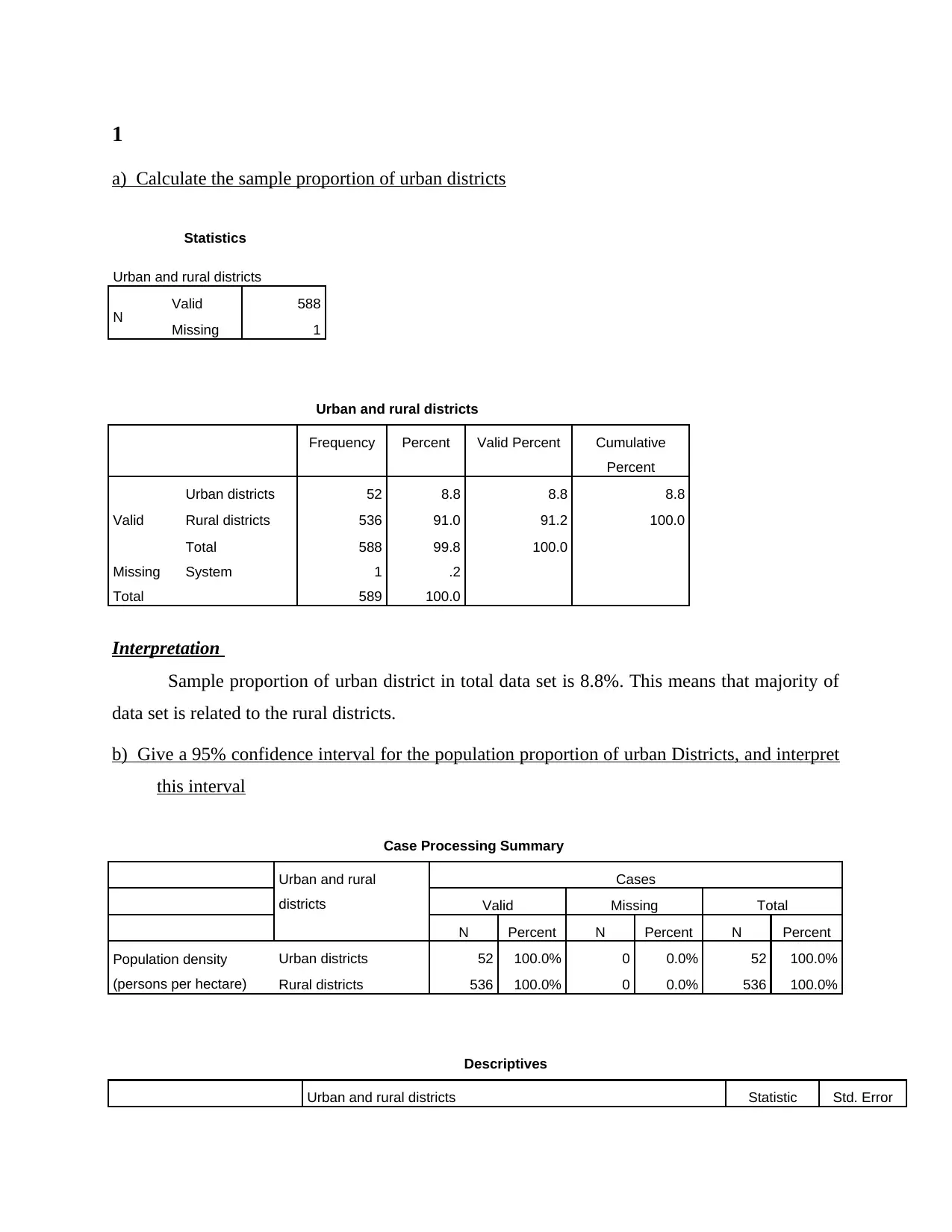
1
a) Calculate the sample proportion of urban districts
Statistics
Urban and rural districts
N Valid 588
Missing 1
Urban and rural districts
Frequency Percent Valid Percent Cumulative
Percent
Valid
Urban districts 52 8.8 8.8 8.8
Rural districts 536 91.0 91.2 100.0
Total 588 99.8 100.0
Missing System 1 .2
Total 589 100.0
Interpretation
Sample proportion of urban district in total data set is 8.8%. This means that majority of
data set is related to the rural districts.
b) Give a 95% confidence interval for the population proportion of urban Districts, and interpret
this interval
Case Processing Summary
Urban and rural
districts
Cases
Valid Missing Total
N Percent N Percent N Percent
Population density
(persons per hectare)
Urban districts 52 100.0% 0 0.0% 52 100.0%
Rural districts 536 100.0% 0 0.0% 536 100.0%
Descriptives
Urban and rural districts Statistic Std. Error

Population density (persons
per hectare)
Urban districts
Mean 130.006 22.2760
95% Confidence Interval for
Mean
Lower Bound 85.285
Upper Bound 174.726
5% Trimmed Mean 114.844
Median 50.063
Variance 25803.453
Std. Deviation 160.6345
Minimum 2.6
Maximum 546.2
Range 543.6
Interquartile Range 168.3
Skewness 1.432 .330
Kurtosis .800 .650
Rural districts
Mean 2.466 .5198
95% Confidence Interval for
Mean
Lower Bound 1.445
Upper Bound 3.487
5% Trimmed Mean 1.104
Median .748
Variance 144.797
Std. Deviation 12.0331
Minimum .1
Maximum 197.6
Range 197.5
Interquartile Range .7
Skewness 12.502 .106
Kurtosis 174.546 .211
Interpretation
At 95% confidence interval proportion of the urban area in data set is in the range of 85-
174. This means that if mean, median and mode of urban area will be 130, 50 and 160 with 95%
confidence then there is a probability that proportion of the urban population in data set of 587
will be in range of 85-174.

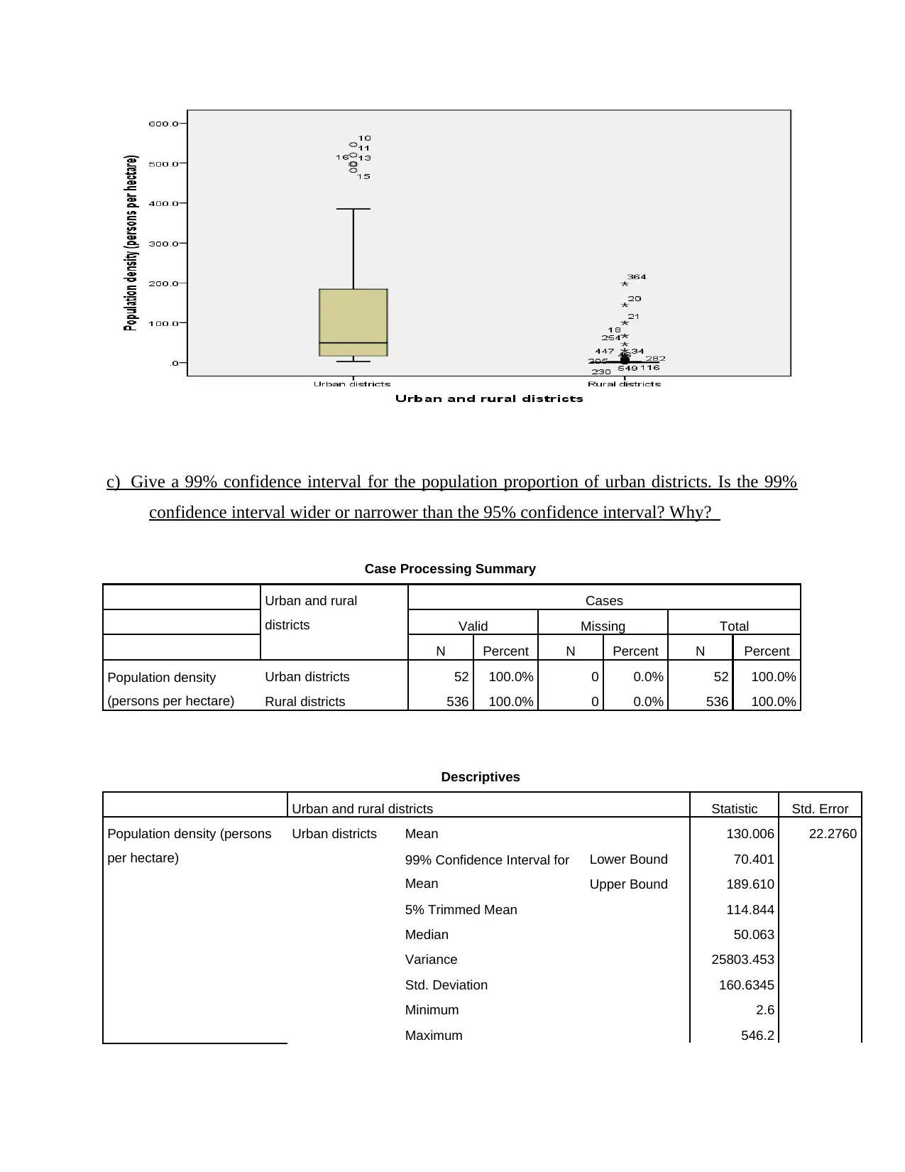
c) Give a 99% confidence interval for the population proportion of urban districts. Is the 99%
confidence interval wider or narrower than the 95% confidence interval? Why?
Case Processing Summary
Urban and rural
districts
Cases
Valid Missing Total
N Percent N Percent N Percent
Population density
(persons per hectare)
Urban districts 52 100.0% 0 0.0% 52 100.0%
Rural districts 536 100.0% 0 0.0% 536 100.0%
Descriptives
Urban and rural districts Statistic Std. Error
Population density (persons
per hectare)
Urban districts Mean 130.006 22.2760
99% Confidence Interval for
Mean
Lower Bound 70.401
Upper Bound 189.610
5% Trimmed Mean 114.844
Median 50.063
Variance 25803.453
Std. Deviation 160.6345
Minimum 2.6
Maximum 546.2

Range 543.6
Interquartile Range 168.3
Skewness 1.432 .330
Kurtosis .800 .650
Rural districts
Mean 2.466 .5198
99% Confidence Interval for
Mean
Lower Bound 1.122
Upper Bound 3.810
5% Trimmed Mean 1.104
Median .748
Variance 144.797
Std. Deviation 12.0331
Minimum .1
Maximum 197.6
Range 197.5
Interquartile Range .7
Skewness 12.502 .106
Kurtosis 174.546 .211
Interpretation
At 99% confidence interval the range of the population of urban districts 74-189. At 99%
confidence interval population range is wide. This happened because by selecting 99%
confidence interval strong believe is shown on the repetition of the mean, median, mode and
standard deviation values. Hence, range of population is wide in case of 99% then 95%
confidence interval.

2
Statistics
Man
N Valid 584
Missing 5
Mean 1.3938
Median 1.0000
Mode 1.00
Percentiles 50 1.0000
Man
Frequency Percent Valid Percent Cumulative
Percent
Valid
Low 385 65.4 65.9 65.9
Medium 168 28.5 28.8 94.7
High 31 5.3 5.3 100.0
Total 584 99.2 100.0
Missing System 5 .8
Total 589 100.0
Interpretation
Research results revealed that there higher percentage of men employed in the manufacturing
sector is 5.3% in the data set. 28% districts have a medium percentage of the people at age
of 20 or above this age group that are employed in the manufacturing sector. Apart from
this, there are 65.9% districts that have youngsters at age of 20 or above that are employed
in the manufacturing sector. Hence, it can be said that in only 5% districts of the sample
there are higher number of people that are working the manufacturing sector.
3
Case Processing Summary
Urban and rural
districts
Cases
Valid Missing Total
N Percent N Percent N Percent
Urban districts 52 100.0% 0 0.0% 52 100.0%

Death rate from phthisis
during 1850s Rural districts 536 100.0% 0 0.0% 536 100.0%
Descriptives
Urban and rural districts Statistic Std. Error
Death rate from phthisis
during 1850s
Urban districts
Mean 2.8640 .08576
99% Confidence Interval for
Mean
Lower Bound 2.6345
Upper Bound 3.0935
5% Trimmed Mean 2.8479
Median 2.8073
Variance .382
Std. Deviation .61844
Minimum 1.55
Maximum 5.10
Range 3.55
Interquartile Range .71
Skewness .702 .330
Kurtosis 2.485 .650
Rural districts
Mean 2.4754 .02232
99% Confidence Interval for
Mean
Lower Bound 2.4177
Upper Bound 2.5331
5% Trimmed Mean 2.4472
Median 2.3957
Variance .267
Std. Deviation .51675
Minimum 1.23
Maximum 5.02
Range 3.79
Interquartile Range .67
Skewness .906 .106
Kurtosis 1.631 .211
Interpretation
The above table which shows the descriptive statistical tools in order to assess the
efficiency of the data obtained throughout the research. The above research is based on
comparison among the urban and rural areas which is assessing the death rates from phthisis

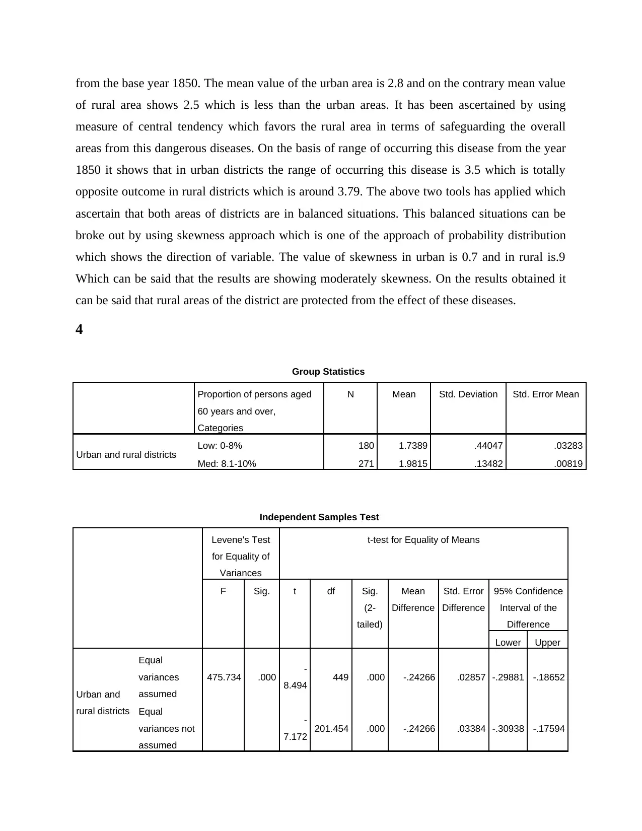
from the base year 1850. The mean value of the urban area is 2.8 and on the contrary mean value
of rural area shows 2.5 which is less than the urban areas. It has been ascertained by using
measure of central tendency which favors the rural area in terms of safeguarding the overall
areas from this dangerous diseases. On the basis of range of occurring this disease from the year
1850 it shows that in urban districts the range of occurring this disease is 3.5 which is totally
opposite outcome in rural districts which is around 3.79. The above two tools has applied which
ascertain that both areas of districts are in balanced situations. This balanced situations can be
broke out by using skewness approach which is one of the approach of probability distribution
which shows the direction of variable. The value of skewness in urban is 0.7 and in rural is.9
Which can be said that the results are showing moderately skewness. On the results obtained it
can be said that rural areas of the district are protected from the effect of these diseases.
4
Group Statistics
Proportion of persons aged
60 years and over,
Categories
N Mean Std. Deviation Std. Error Mean
Urban and rural districts Low: 0-8% 180 1.7389 .44047 .03283
Med: 8.1-10% 271 1.9815 .13482 .00819
Independent Samples Test
Levene's Test
for Equality of
Variances
t-test for Equality of Means
F Sig. t df Sig.
(2-
tailed)
Mean
Difference
Std. Error
Difference
95% Confidence
Interval of the
Difference
Lower Upper
Urban and
rural districts
Equal
variances
assumed
475.734 .000 -
8.494 449 .000 -.24266 .02857 -.29881 -.18652
Equal
variances not
assumed
-
7.172 201.454 .000 -.24266 .03384 -.30938 -.17594

Interpretation
The above comparison is based on the ascertaining the proportion of people aged above 60 years
from which of the particular district whether it was urban or rural. The above comparison is
based on applying leven test for equality of variances. The sign value less than 0.5 shows the
score of one variable is different from one another which shows the deficiency of the results. The
above value of sign 2 tailed are less than 0.5 which shows that the means of both the variables
are not likely to change from one period to another. The decision of selecting a proportion of
people age above 60 years will be based on the group statistics. This States that both the
variables have different number of conditions and their decision will be based on the mean. The
mean value says that rural districts will have higher mean value along with the higher number of
conditions.
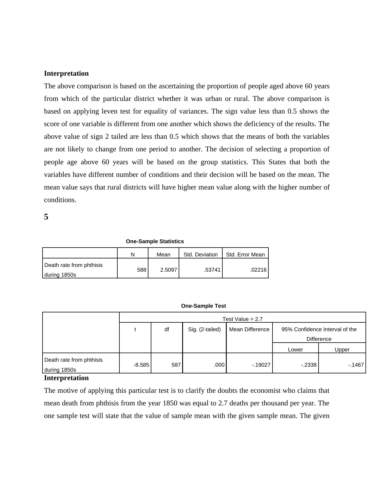
5
One-Sample Statistics
N Mean Std. Deviation Std. Error Mean
Death rate from phthisis
during 1850s 588 2.5097 .53741 .02216
One-Sample Test
Test Value = 2.7
t df Sig. (2-tailed) Mean Difference 95% Confidence Interval of the
Difference
Lower Upper
Death rate from phthisis
during 1850s -8.585 587 .000 -.19027 -.2338 -.1467
Interpretation
The motive of applying this particular test is to clarify the doubts the economist who claims that
mean death from phthisis from the year 1850 was equal to 2.7 deaths per thousand per year. The
one sample test will state that the value of sample mean with the given sample mean. The given

mean is 2.7 and the actual mean obtained is 2.5. The claim of the economist is wrong as standard
mean is less than the actual mean generated.
6
ANOVA
Death rate from phthisis during 1850s
Sum of Squares df Mean Square F Sig.
Between Groups 168.662 578 .292 3.030 .035
Within Groups .867 9 .096
Total 169.529 587
Interpretation
The above annova technique has applied by an enterprise in assessing the complete
direction of between the two years of 1850 and 1870. The decision s will be based on the sum of
squares and mean of squares. The group which has both the higher values is between groups
values death are lies between the year of 1850 and 1870.
7
ANOVA
Death
Sum of Squares df Mean Square F Sig.
Between Groups 3.252 1 3.252 7.815 .008
Within Groups 18.308 44 .416
Total 21.560 45
Interpretation
The above technique has applied in order to identify the difference between two cities
such as Hampshire and New South Wales which means that there is a significant difference
between the both variables.

TASK 2
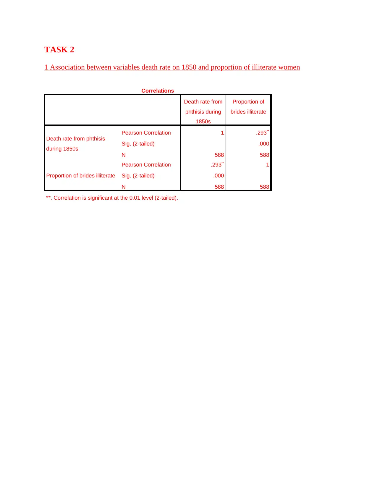
1 Association between variables death rate on 1850 and proportion of illiterate women
Correlations
Death rate from
phthisis during
1850s
Proportion of
brides illiterate
Death rate from phthisis
during 1850s
Pearson Correlation 1 .293**
Sig. (2-tailed) .000
N 588 588
Proportion of brides illiterate
Pearson Correlation .293** 1
Sig. (2-tailed) .000
N 588 588
**. Correlation is significant at the 0.01 level (2-tailed).

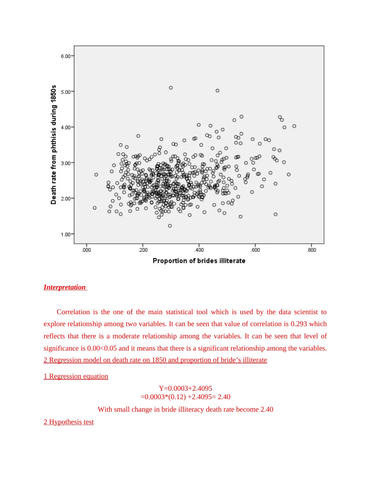
Interpretation
Correlation is the one of the main statistical tool which is used by the data scientist to
explore relationship among two variables. It can be seen that value of correlation is 0.293 which
reflects that there is a moderate relationship among the variables. It can be seen that level of
significance is 0.00<0.05 and it means that there is a significant relationship among the variables.
2 Regression model on death rate on 1850 and proportion of bride’s illiterate
1 Regression equation
Y=0.0003+2.4095
=0.0003*(0.12) +2.4095= 2.40
With small change in bride illiteracy death rate become 2.40
2 Hypothesis test

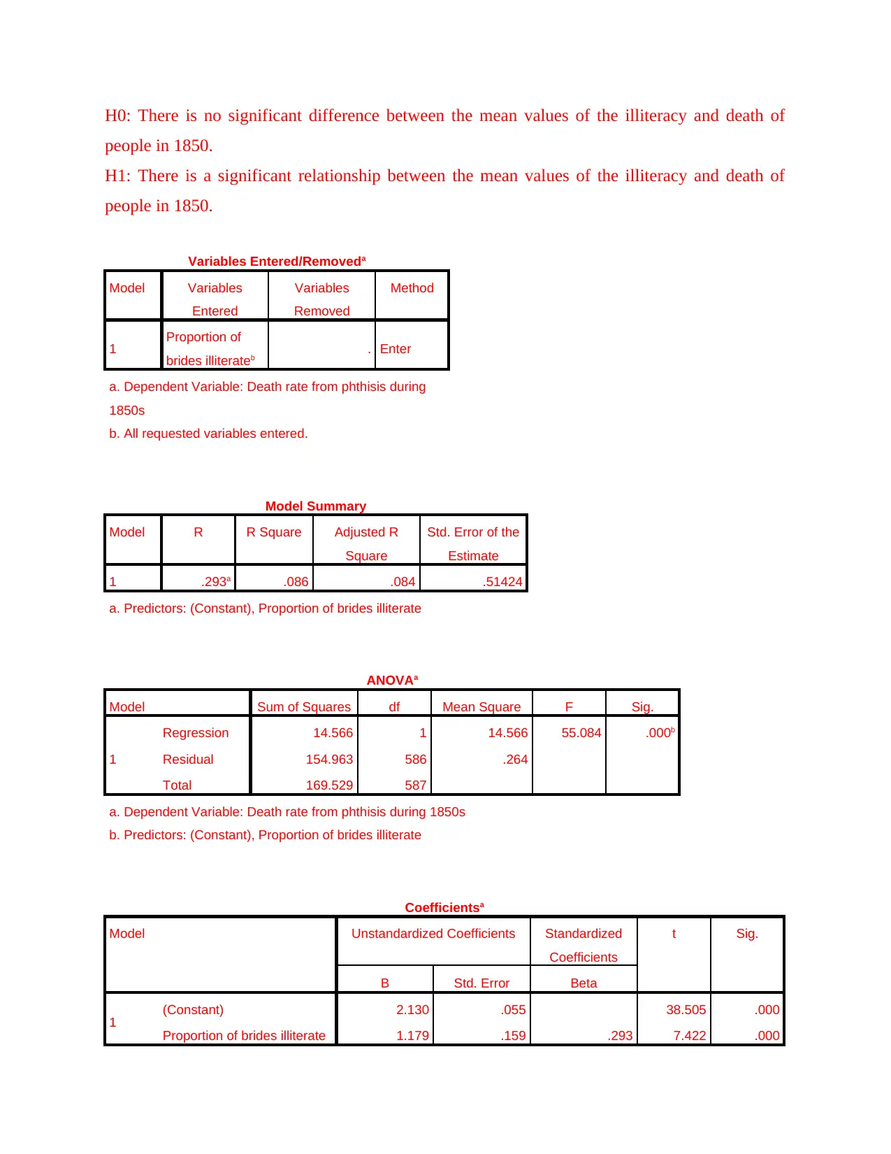
H0: There is no significant difference between the mean values of the illiteracy and death of
people in 1850.
H1: There is a significant relationship between the mean values of the illiteracy and death of
people in 1850.
Variables Entered/Removeda
Model Variables
Entered
Variables
Removed
Method
1 Proportion of
brides illiterateb . Enter
a. Dependent Variable: Death rate from phthisis during
1850s
b. All requested variables entered.
Model Summary
Model R R Square Adjusted R
Square
Std. Error of the
Estimate
1 .293a .086 .084 .51424
a. Predictors: (Constant), Proportion of brides illiterate
ANOVAa
Model Sum of Squares df Mean Square F Sig.
1
Regression 14.566 1 14.566 55.084 .000b
Residual 154.963 586 .264
Total 169.529 587
a. Dependent Variable: Death rate from phthisis during 1850s
b. Predictors: (Constant), Proportion of brides illiterate
Coefficientsa
Model Unstandardized Coefficients Standardized
Coefficients
t Sig.
B Std. Error Beta
1 (Constant) 2.130 .055 38.505 .000
Proportion of brides illiterate 1.179 .159 .293 7.422 .000

a. Dependent Variable: Death rate from phthisis during 1850s
Interpretation
On the basis of results of the regression model it is interpreted that there is a significant
difference in the mean values of the death of people 1850 and illiteracy of brides. This tool is
used for analysis purpose because by using it can be identified that with change in the dependent
variable what change comes in the independent variable.
3 Prediction of death rate from parenthesis
Death rate from parenthesis will be 2.40 if bride illiteracy get change slightly. Hence, it
can be said that illiteracy affects the death rate from parenthesis.
4 Regression model at 99% confidence interval
Variables Entered/Removeda
Model Variables
Entered
Variables
Removed
Method
1 Proportion of
brides illiterateb . Enter
a. Dependent Variable: Death rate from phthisis during
1850s
b. All requested variables entered.
Model Summary
Model R R Square Adjusted R
Square
Std. Error of the
Estimate
1 .293a .086 .084 .51424
a. Predictors: (Constant), Proportion of brides illiterate
ANOVAa
Model Sum of Squares df Mean Square F Sig.
1
Regression 14.566 1 14.566 55.084 .000b
Residual 154.963 586 .264
Total 169.529 587
a. Dependent Variable: Death rate from phthisis during 1850s

b. Predictors: (Constant), Proportion of brides illiterate
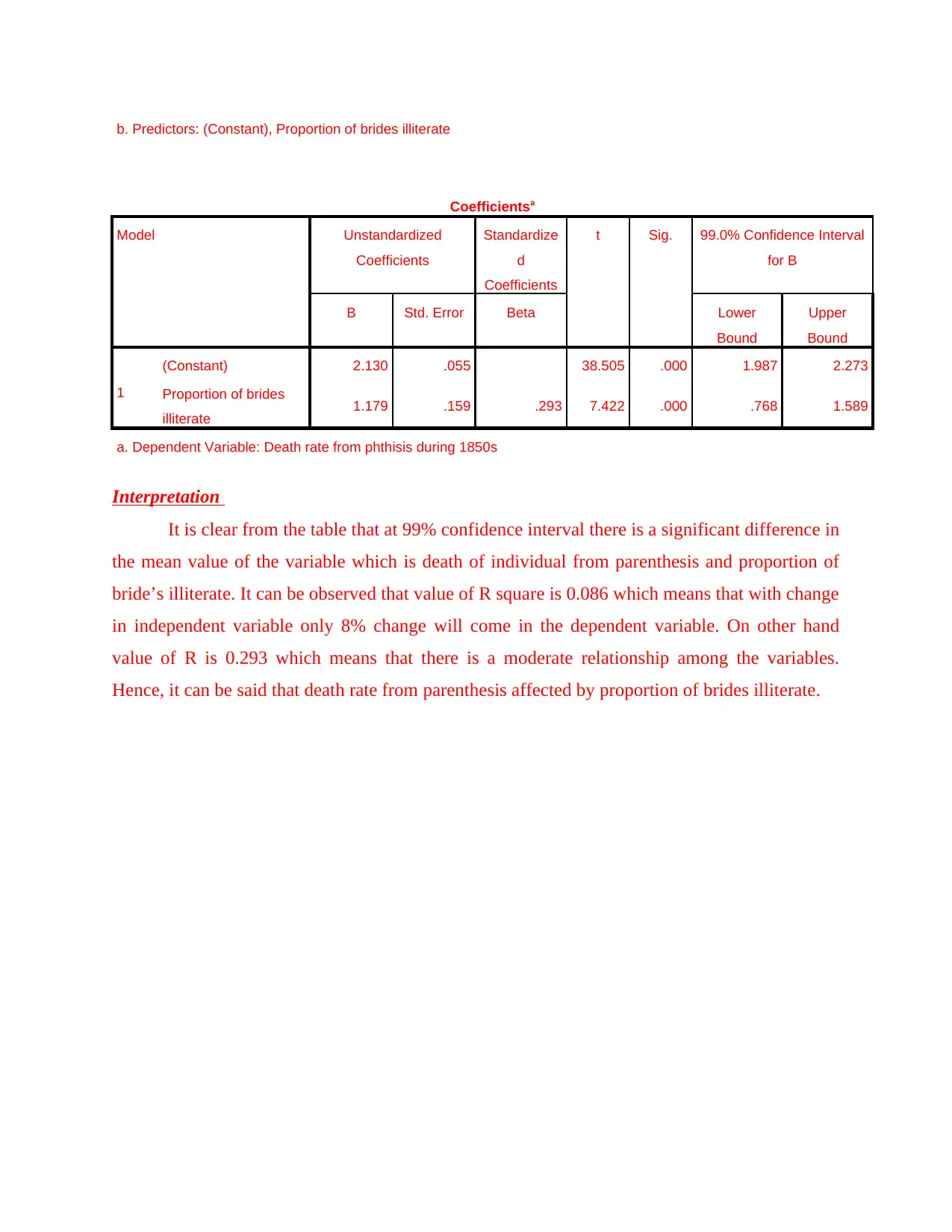
Coefficientsa
Model Unstandardized
Coefficients
Standardize
d
Coefficients
t Sig. 99.0% Confidence Interval
for B
B Std. Error Beta Lower
Bound
Upper
Bound
1
(Constant) 2.130 .055 38.505 .000 1.987 2.273
Proportion of brides
illiterate 1.179 .159 .293 7.422 .000 .768 1.589
a. Dependent Variable: Death rate from phthisis during 1850s
Interpretation
It is clear from the table that at 99% confidence interval there is a significant difference in
the mean value of the variable which is death of individual from parenthesis and proportion of
bride’s illiterate. It can be observed that value of R square is 0.086 which means that with change
in independent variable only 8% change will come in the dependent variable. On other hand
value of R is 0.293 which means that there is a moderate relationship among the variables.
Hence, it can be said that death rate from parenthesis affected by proportion of brides illiterate.

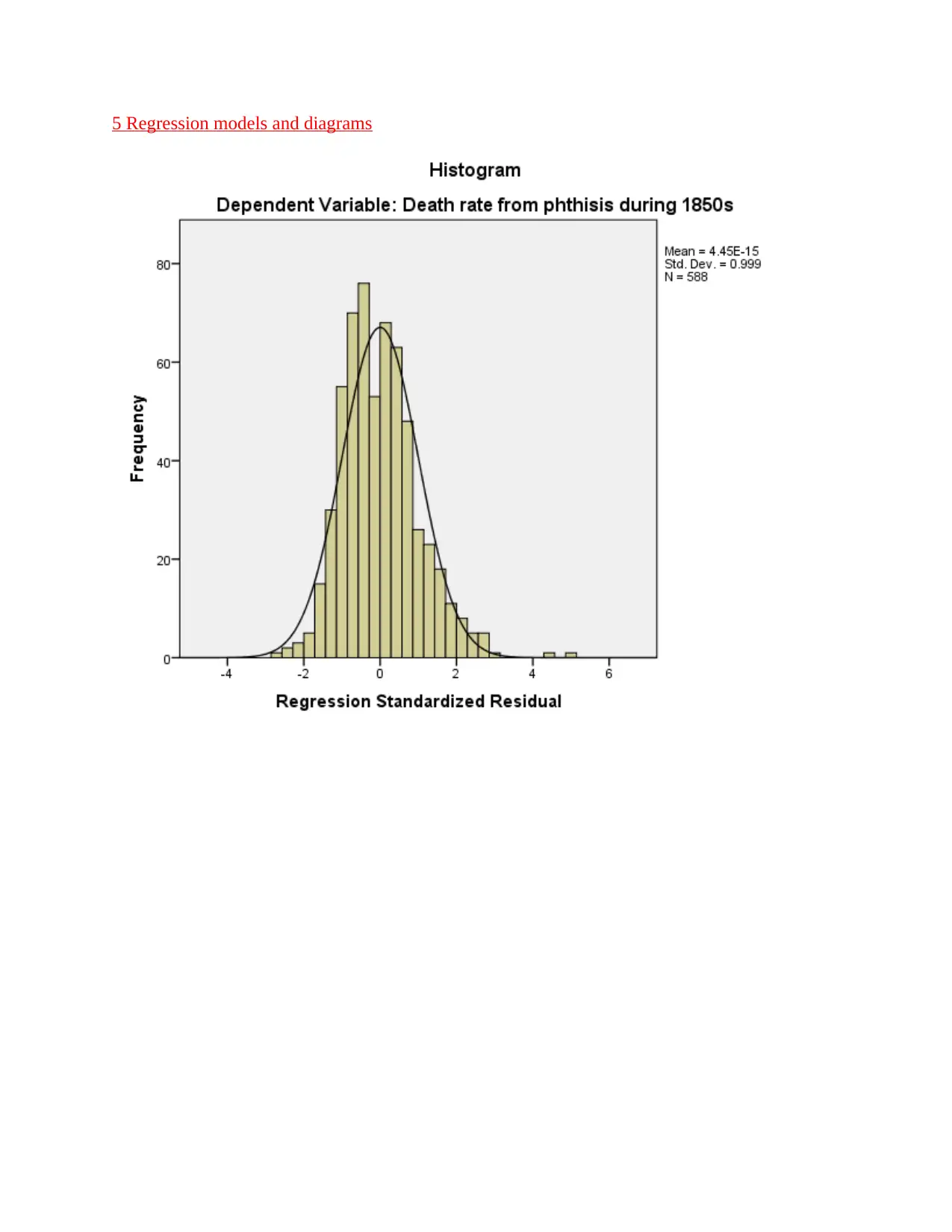
5 Regression models and diagrams

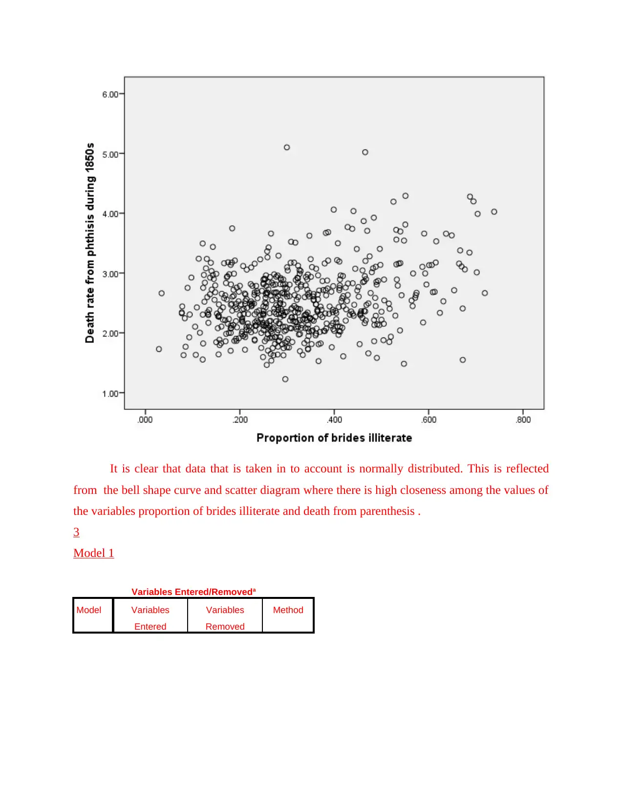
It is clear that data that is taken in to account is normally distributed. This is reflected
from the bell shape curve and scatter diagram where there is high closeness among the values of
the variables proportion of brides illiterate and death from parenthesis .
3
Model 1
Variables Entered/Removeda
Model Variables
Entered
Variables
Removed
Method

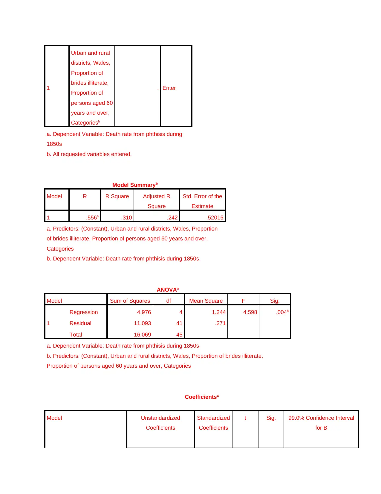
1
Urban and rural
districts, Wales,
Proportion of
brides illiterate,
Proportion of
persons aged 60
years and over,
Categoriesb
. Enter
a. Dependent Variable: Death rate from phthisis during
1850s
b. All requested variables entered.
Model Summaryb
Model R R Square Adjusted R
Square
Std. Error of the
Estimate
1 .556a .310 .242 .52015
a. Predictors: (Constant), Urban and rural districts, Wales, Proportion
of brides illiterate, Proportion of persons aged 60 years and over,
Categories
b. Dependent Variable: Death rate from phthisis during 1850s
ANOVAa
Model Sum of Squares df Mean Square F Sig.
1
Regression 4.976 4 1.244 4.598 .004b
Residual 11.093 41 .271
Total 16.069 45
a. Dependent Variable: Death rate from phthisis during 1850s
b. Predictors: (Constant), Urban and rural districts, Wales, Proportion of brides illiterate,
Proportion of persons aged 60 years and over, Categories
Coefficientsa
Model Unstandardized
Coefficients
Standardized
Coefficients
t Sig. 99.0% Confidence Interval
for B

B Std. Error Beta Lower Bound Upper Bound
1
(Constant) 3.127 .328 9.520 .000 2.240 4.014
Proportion of brides
illiterate 1.851 .932 .278 1.987 .054 -.665 4.367
Wales -.218 .410 -.075 -.533 .597 -1.325 .888
Proportion of persons
aged 60 years and
over, Categories
.004 .213 .003 .020 .984 -.570 .579
Urban and rural
districts -.641 .179 -.542 -3.585 .001 -1.124 -.158
a. Dependent Variable: Death rate from phthisis during 1850s
Residuals Statisticsa
Minimum Maximum Mean Std. Deviation N
Predicted Value 1.9227 3.2772 2.5331 .33254 46
Residual -1.01238 1.31830 .00000 .49649 46
Std. Predicted Value -1.835 2.238 .000 1.000 46
Std. Residual -1.946 2.534 .000 .955 46
a. Dependent Variable: Death rate from phthisis during 1850s

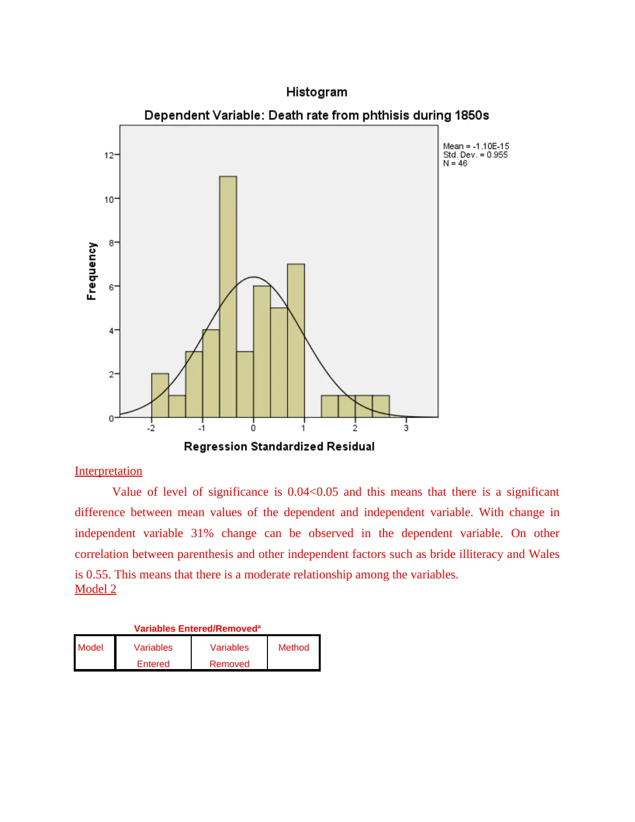
Interpretation
Value of level of significance is 0.04<0.05 and this means that there is a significant
difference between mean values of the dependent and independent variable. With change in
independent variable 31% change can be observed in the dependent variable. On other
correlation between parenthesis and other independent factors such as bride illiteracy and Wales
is 0.55. This means that there is a moderate relationship among the variables.
Model 2
Variables Entered/Removeda
Model Variables
Entered
Variables
Removed
Method

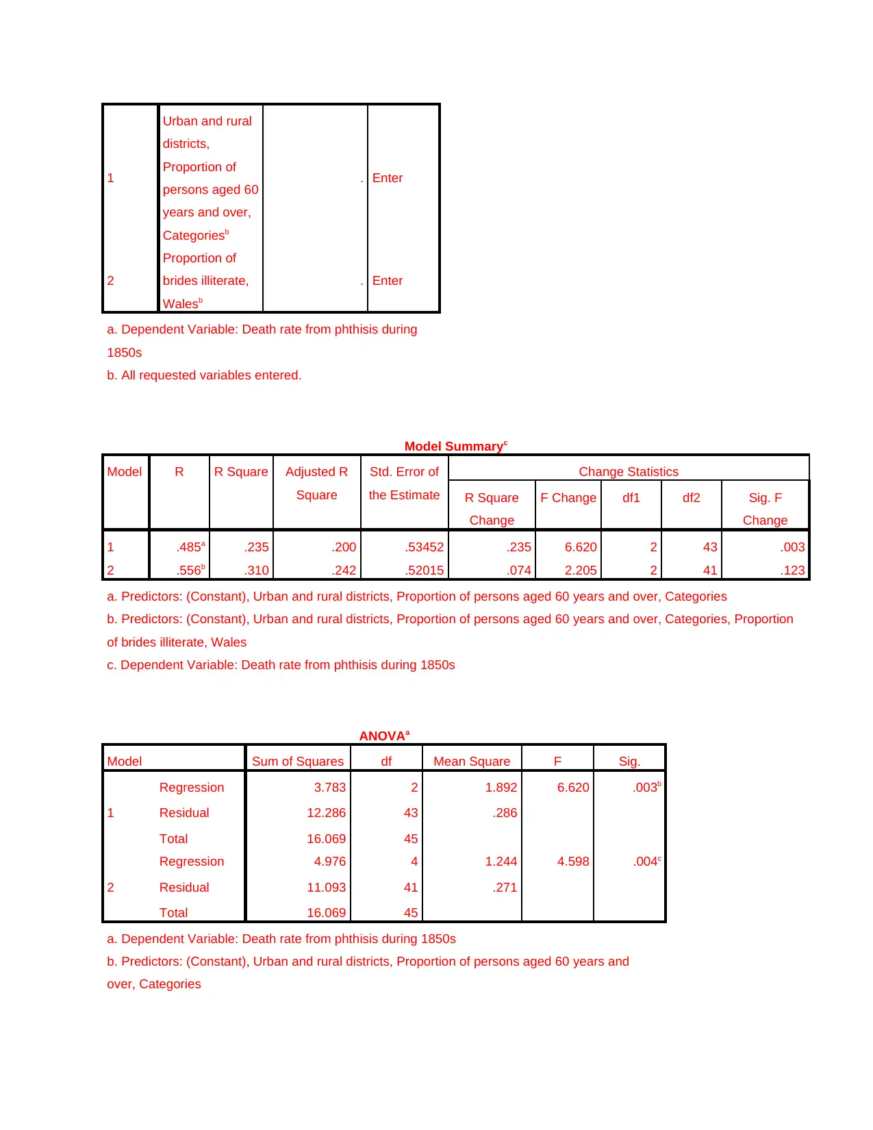
1
Urban and rural
districts,
Proportion of
persons aged 60
years and over,
Categoriesb
. Enter
2
Proportion of
brides illiterate,
Walesb
. Enter
a. Dependent Variable: Death rate from phthisis during
1850s
b. All requested variables entered.
Model Summaryc
Model R R Square Adjusted R
Square
Std. Error of
the Estimate
Change Statistics
R Square
Change
F Change df1 df2 Sig. F
Change
1 .485a .235 .200 .53452 .235 6.620 2 43 .003
2 .556b .310 .242 .52015 .074 2.205 2 41 .123
a. Predictors: (Constant), Urban and rural districts, Proportion of persons aged 60 years and over, Categories
b. Predictors: (Constant), Urban and rural districts, Proportion of persons aged 60 years and over, Categories, Proportion
of brides illiterate, Wales
c. Dependent Variable: Death rate from phthisis during 1850s
ANOVAa
Model Sum of Squares df Mean Square F Sig.
1
Regression 3.783 2 1.892 6.620 .003b
Residual 12.286 43 .286
Total 16.069 45
2
Regression 4.976 4 1.244 4.598 .004c
Residual 11.093 41 .271
Total 16.069 45
a. Dependent Variable: Death rate from phthisis during 1850s
b. Predictors: (Constant), Urban and rural districts, Proportion of persons aged 60 years and
over, Categories

c. Predictors: (Constant), Urban and rural districts, Proportion of persons aged 60 years and over,
Categories, Proportion of brides illiterate, Wales
Coefficientsa
Model Unstandardized
Coefficients
Standardize
d
Coefficients
t Sig. 99.0% Confidence Interval
for B
B Std. Error Beta Lower
Bound
Upper
Bound
1
(Constant) 3.485 .288 12.099 .000 2.709 4.262
Proportion of persons
aged 60 years and
over, Categories
-.151 .195 -.112 -.771 .445 -.678 .376
Urban and rural
districts -.508 .172 -.430 -2.960 .005 -.971 -.045
2
(Constant) 3.127 .328 9.520 .000 2.240 4.014
Proportion of persons
aged 60 years and
over, Categories
.004 .213 .003 .020 .984 -.570 .579
Urban and rural
districts -.641 .179 -.542 -3.585 .001 -1.124 -.158
Proportion of brides
illiterate 1.851 .932 .278 1.987 .054 -.665 4.367
Wales -.218 .410 -.075 -.533 .597 -1.325 .888
a. Dependent Variable: Death rate from phthisis during 1850s
Excluded Variablesa
Model Beta In t Sig. Partial
Correlation
Collinearity
Statistics
Tolerance
1 Proportion of brides illiterate .283b 2.049 .047 .301 .866
Wales -.096b -.656 .515 -.101 .847