STA10008 Foundations of Statistics Project - B | Desklib

The article is about a project related to the study of Australian adolescents in 2020. It includes data preparation, questions, and their solutions using SPSS. The questions include one-sample t-test, independent samples t-test, paired samples t-test, and regression analysis. The article also includes the assumptions and relevant output for each question.

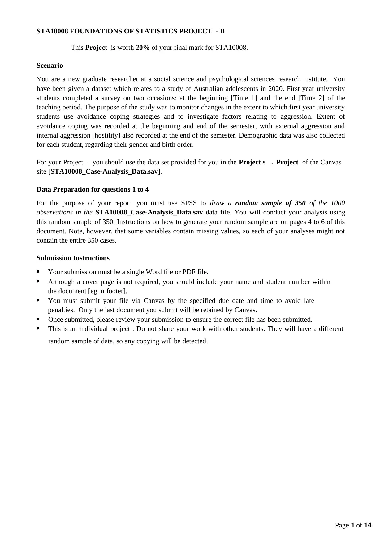
STA10008 FOUNDATIONS OF STATISTICS PROJECT - B
This Project is worth 20% of your final mark for STA10008.
Scenario
You are a new graduate researcher at a social science and psychological sciences research institute. You
have been given a dataset which relates to a study of Australian adolescents in 2020. First year university
students completed a survey on two occasions: at the beginning [Time 1] and the end [Time 2] of the
teaching period. The purpose of the study was to monitor changes in the extent to which first year university
students use avoidance coping strategies and to investigate factors relating to aggression. Extent of
avoidance coping was recorded at the beginning and end of the semester, with external aggression and
internal aggression [hostility] also recorded at the end of the semester. Demographic data was also collected
for each student, regarding their gender and birth order.
For your Project – you should use the data set provided for you in the Project s → Project of the Canvas
site [STA10008_Case-Analysis_Data.sav].
Data Preparation for questions 1 to 4
For the purpose of your report, you must use SPSS to draw a random sample of 350 of the 1000
observations in the STA10008_Case-Analysis_Data.sav data file. You will conduct your analysis using
this random sample of 350. Instructions on how to generate your random sample are on pages 4 to 6 of this
document. Note, however, that some variables contain missing values, so each of your analyses might not
contain the entire 350 cases.
Submission Instructions
 Your submission must be a single Word file or PDF file.
 Although a cover page is not required, you should include your name and student number within
the document [eg in footer].
 You must submit your file via Canvas by the specified due date and time to avoid late
penalties. Only the last document you submit will be retained by Canvas.
 Once submitted, please review your submission to ensure the correct file has been submitted.
 This is an individual project . Do not share your work with other students. They will have a different
random sample of data, so any copying will be detected.
Page 1 of 14

For each of requiring SPSS [Q1 to Q4], you should include the relevant output [eg tables and graphs] with
your report. You are also required to complete question 5 and 6, containing short answer questions.
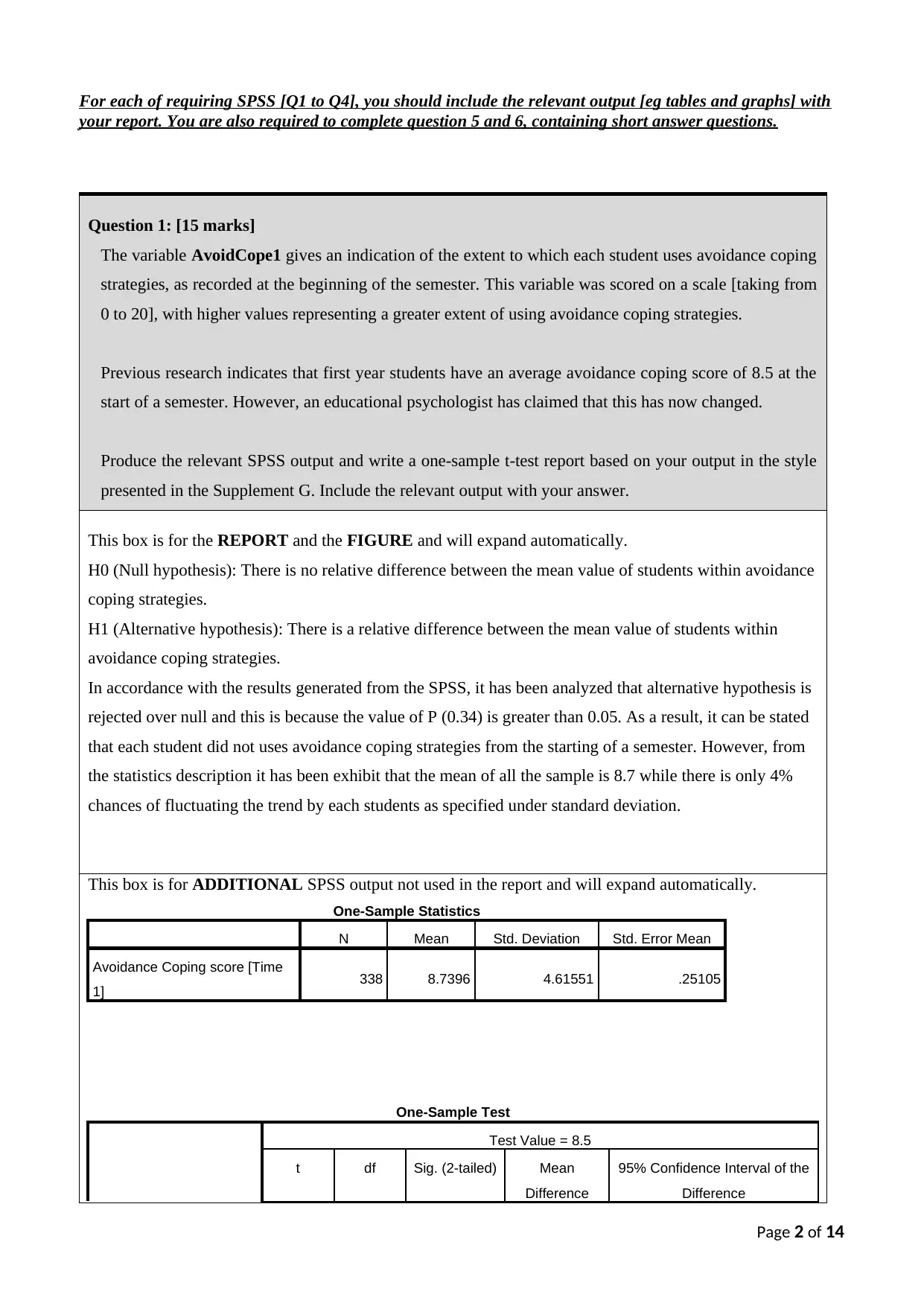
Question 1: [15 marks]
The variable AvoidCope1 gives an indication of the extent to which each student uses avoidance coping
strategies, as recorded at the beginning of the semester. This variable was scored on a scale [taking from
0 to 20], with higher values representing a greater extent of using avoidance coping strategies.
Previous research indicates that first year students have an average avoidance coping score of 8.5 at the
start of a semester. However, an educational psychologist has claimed that this has now changed.
Produce the relevant SPSS output and write a one-sample t-test report based on your output in the style
presented in the Supplement G. Include the relevant output with your answer.
This box is for the REPORT and the FIGURE and will expand automatically.
H0 (Null hypothesis): There is no relative difference between the mean value of students within avoidance
coping strategies.
H1 (Alternative hypothesis): There is a relative difference between the mean value of students within
avoidance coping strategies.
In accordance with the results generated from the SPSS, it has been analyzed that alternative hypothesis is
rejected over null and this is because the value of P (0.34) is greater than 0.05. As a result, it can be stated
that each student did not uses avoidance coping strategies from the starting of a semester. However, from
the statistics description it has been exhibit that the mean of all the sample is 8.7 while there is only 4%
chances of fluctuating the trend by each students as specified under standard deviation.
This box is for ADDITIONAL SPSS output not used in the report and will expand automatically.
One-Sample Statistics
N Mean Std. Deviation Std. Error Mean
Avoidance Coping score [Time
1] 338 8.7396 4.61551 .25105
One-Sample Test
Test Value = 8.5
t df Sig. (2-tailed) Mean
Difference
95% Confidence Interval of the
Difference
Page 2 of 14

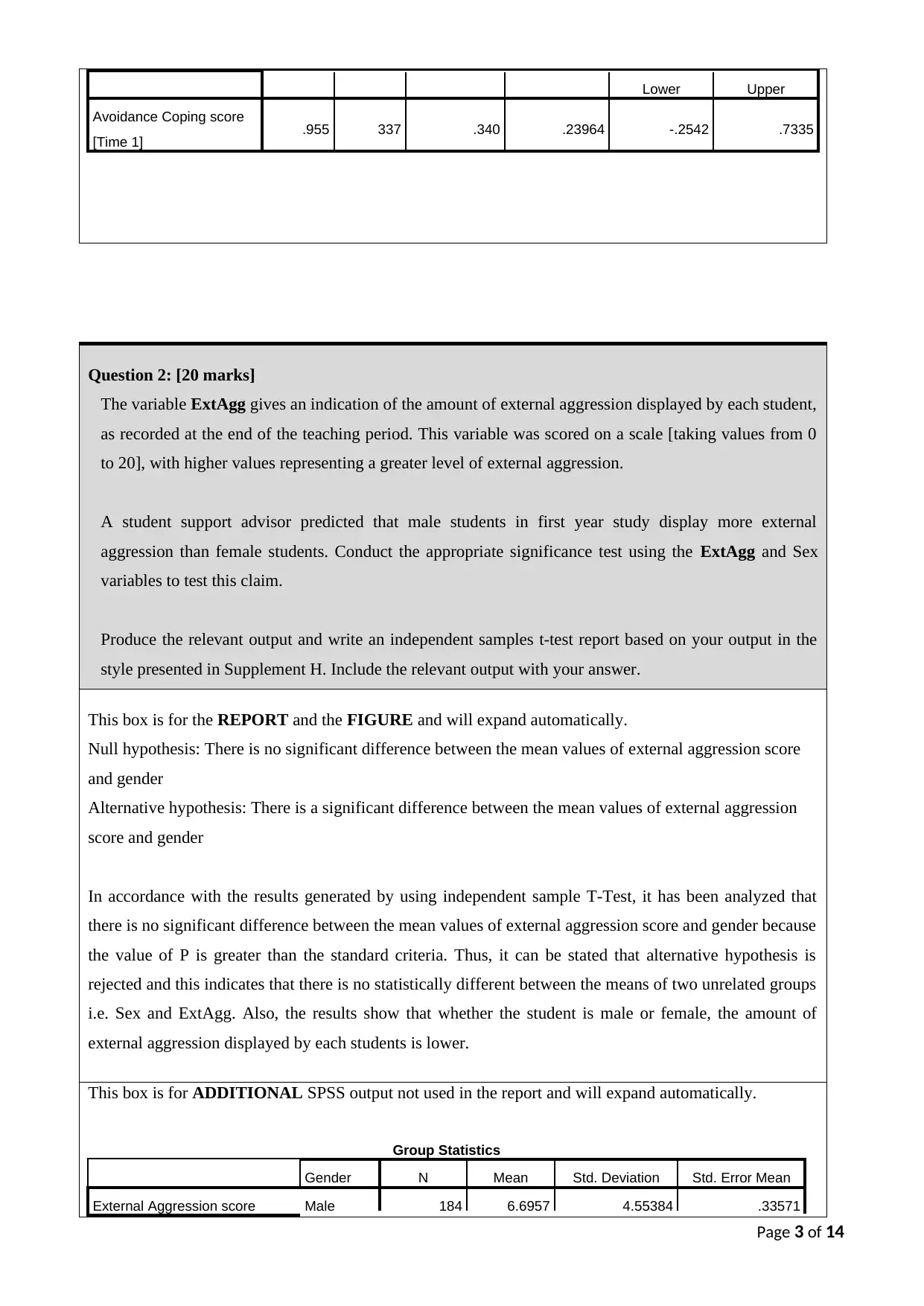
Lower Upper
Avoidance Coping score
[Time 1] .955 337 .340 .23964 -.2542 .7335
Question 2: [20 marks]
The variable ExtAgg gives an indication of the amount of external aggression displayed by each student,
as recorded at the end of the teaching period. This variable was scored on a scale [taking values from 0
to 20], with higher values representing a greater level of external aggression.
A student support advisor predicted that male students in first year study display more external
aggression than female students. Conduct the appropriate significance test using the ExtAgg and Sex
variables to test this claim.
Produce the relevant output and write an independent samples t-test report based on your output in the
style presented in Supplement H. Include the relevant output with your answer.
This box is for the REPORT and the FIGURE and will expand automatically.
Null hypothesis: There is no significant difference between the mean values of external aggression score
and gender
Alternative hypothesis: There is a significant difference between the mean values of external aggression
score and gender
In accordance with the results generated by using independent sample T-Test, it has been analyzed that
there is no significant difference between the mean values of external aggression score and gender because
the value of P is greater than the standard criteria. Thus, it can be stated that alternative hypothesis is
rejected and this indicates that there is no statistically different between the means of two unrelated groups
i.e. Sex and ExtAgg. Also, the results show that whether the student is male or female, the amount of
external aggression displayed by each students is lower.
This box is for ADDITIONAL SPSS output not used in the report and will expand automatically.
Group Statistics
Gender N Mean Std. Deviation Std. Error Mean
External Aggression score Male 184 6.6957 4.55384 .33571
Page 3 of 14

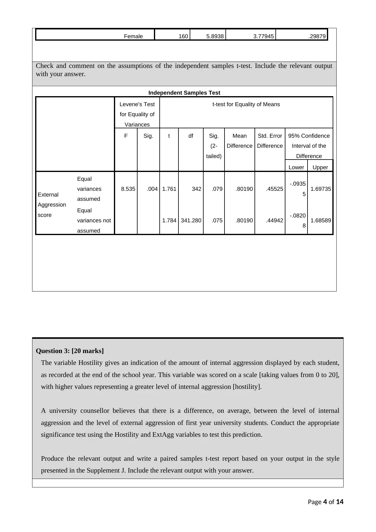
Female 160 5.8938 3.77945 .29879
Check and comment on the assumptions of the independent samples t-test. Include the relevant output
with your answer.
Independent Samples Test
Levene's Test
for Equality of
Variances
t-test for Equality of Means
F Sig. t df Sig.
(2-
tailed)
Mean
Difference
Std. Error
Difference
95% Confidence
Interval of the
Difference
Lower Upper
External
Aggression
score
Equal
variances
assumed
8.535 .004 1.761 342 .079 .80190 .45525 -.0935
5 1.69735
Equal
variances not
assumed
1.784 341.280 .075 .80190 .44942 -.0820
8 1.68589
Question 3: [20 marks]
The variable Hostility gives an indication of the amount of internal aggression displayed by each student,
as recorded at the end of the school year. This variable was scored on a scale [taking values from 0 to 20],
with higher values representing a greater level of internal aggression [hostility].
A university counsellor believes that there is a difference, on average, between the level of internal
aggression and the level of external aggression of first year university students. Conduct the appropriate
significance test using the Hostility and ExtAgg variables to test this prediction.
Produce the relevant output and write a paired samples t-test report based on your output in the style
presented in the Supplement J. Include the relevant output with your answer.
Page 4 of 14

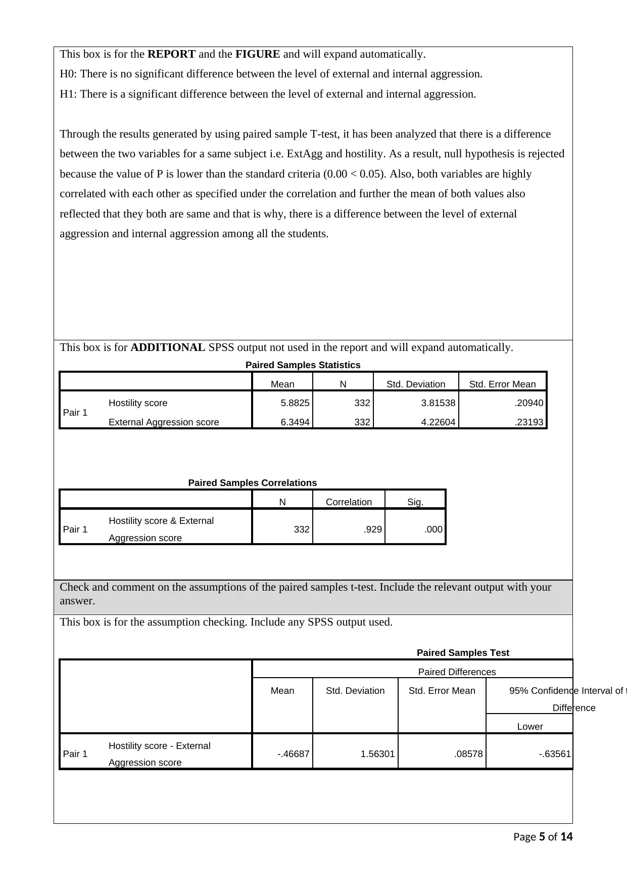
This box is for the REPORT and the FIGURE and will expand automatically.
H0: There is no significant difference between the level of external and internal aggression.
H1: There is a significant difference between the level of external and internal aggression.
Through the results generated by using paired sample T-test, it has been analyzed that there is a difference
between the two variables for a same subject i.e. ExtAgg and hostility. As a result, null hypothesis is rejected
because the value of P is lower than the standard criteria (0.00 < 0.05). Also, both variables are highly
correlated with each other as specified under the correlation and further the mean of both values also
reflected that they both are same and that is why, there is a difference between the level of external
aggression and internal aggression among all the students.
This box is for ADDITIONAL SPSS output not used in the report and will expand automatically.
Paired Samples Statistics
Mean N Std. Deviation Std. Error Mean
Pair 1 Hostility score 5.8825 332 3.81538 .20940
External Aggression score 6.3494 332 4.22604 .23193
Paired Samples Correlations
N Correlation Sig.
Pair 1 Hostility score & External
Aggression score 332 .929 .000
Check and comment on the assumptions of the paired samples t-test. Include the relevant output with your
answer.
This box is for the assumption checking. Include any SPSS output used.
Paired Samples Test
Paired Differences
Mean Std. Deviation Std. Error Mean 95% Confidence Interval of t
Difference
Lower
Pair 1 Hostility score - External
Aggression score -.46687 1.56301 .08578 -.63561
Page 5 of 14

Question 4: [2,3,5,10 marks]
A researcher in early childhood development wanted to know whether children who spend more time
watching television tend to have lower hand-eye co-ordination skills. He selected a random sample of 6-
year-old children and measured their hand-eye co-ordination using a standardised test. He also asked
their parents to record how much time they spent watching television during the week.
Use your random sample taken from STA10008_Case-Analysis_Data.sav to test the researcher’s
hypothesis.
a. What is the dependent variable?
In this, the dependent variable is hand- eye- coordination because such variable is relied upon number of
time spend upon watching television. Therefore, this the coordination of hand and eye will be changes as
per the number of watching hours of TV changes. That is why, it is chosen as a dependent variable.
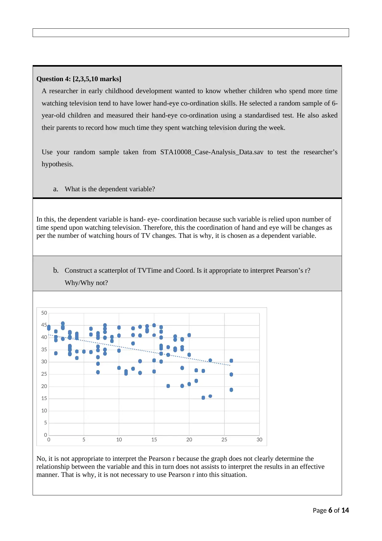
b. Construct a scatterplot of TVTime and Coord. Is it appropriate to interpret Pearson’s r?
Why/Why not?
0 5 10 15 20 25 30
0
5
10
15
20
25
30
35
40
45
50
No, it is not appropriate to interpret the Pearson r because the graph does not clearly determine the
relationship between the variable and this in turn does not assists to interpret the results in an effective
manner. That is why, it is not necessary to use Pearson r into this situation.
Page 6 of 14

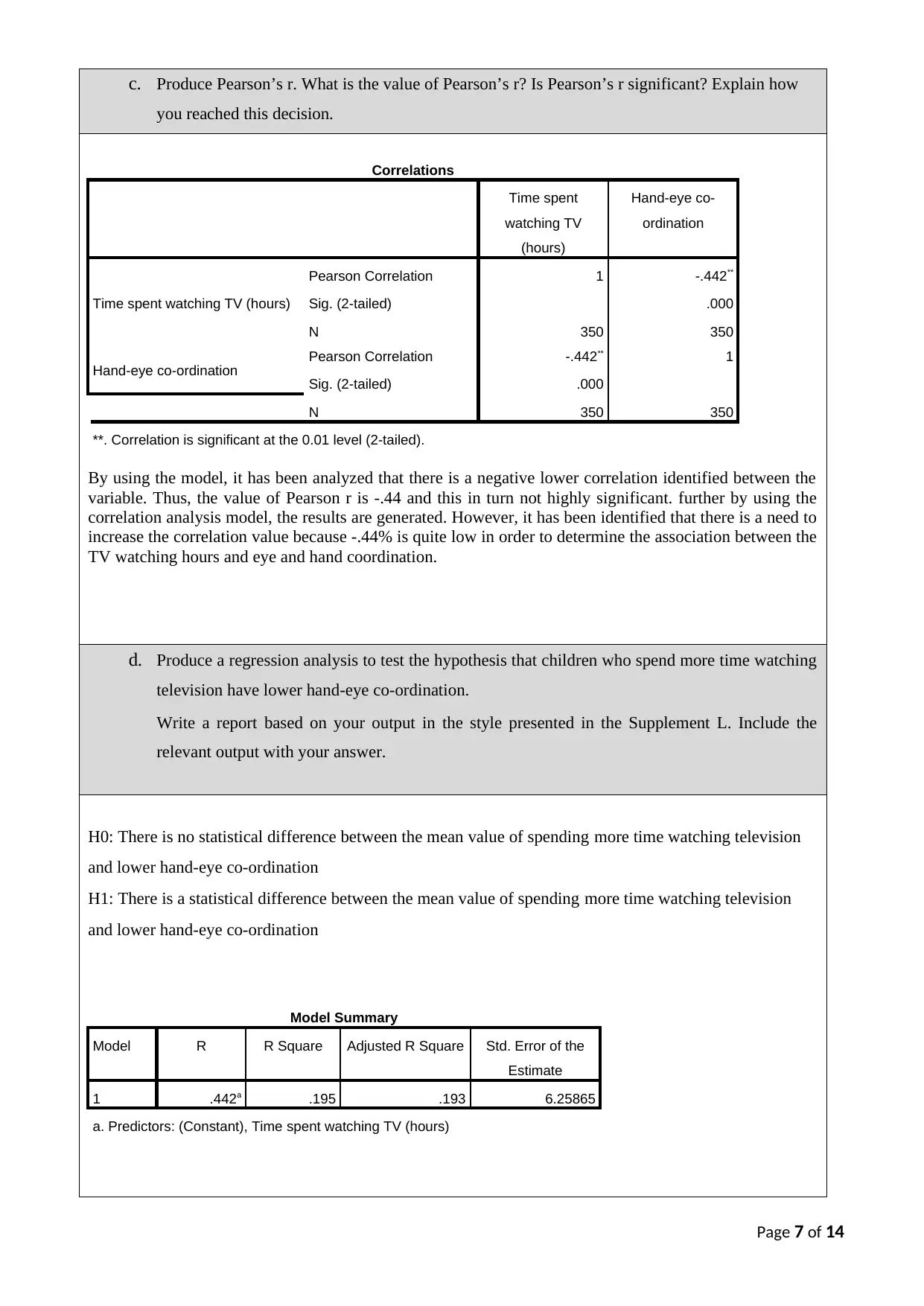
c. Produce Pearson’s r. What is the value of Pearson’s r? Is Pearson’s r significant? Explain how
you reached this decision.
Correlations
Time spent
watching TV
(hours)
Hand-eye co-
ordination
Time spent watching TV (hours)
Pearson Correlation 1 -.442**
Sig. (2-tailed) .000
N 350 350
Hand-eye co-ordination Pearson Correlation -.442** 1
Sig. (2-tailed) .000
N 350 350
**. Correlation is significant at the 0.01 level (2-tailed).
By using the model, it has been analyzed that there is a negative lower correlation identified between the
variable. Thus, the value of Pearson r is -.44 and this in turn not highly significant. further by using the
correlation analysis model, the results are generated. However, it has been identified that there is a need to
increase the correlation value because -.44% is quite low in order to determine the association between the
TV watching hours and eye and hand coordination.
d. Produce a regression analysis to test the hypothesis that children who spend more time watching
television have lower hand-eye co-ordination.
Write a report based on your output in the style presented in the Supplement L. Include the
relevant output with your answer.
H0: There is no statistical difference between the mean value of spending more time watching television
and lower hand-eye co-ordination
H1: There is a statistical difference between the mean value of spending more time watching television
and lower hand-eye co-ordination
Model Summary
Model R R Square Adjusted R Square Std. Error of the
Estimate
1 .442a .195 .193 6.25865
a. Predictors: (Constant), Time spent watching TV (hours)
Page 7 of 14

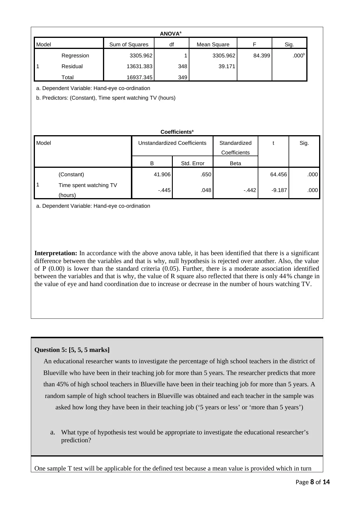
ANOVAa
Model Sum of Squares df Mean Square F Sig.
1
Regression 3305.962 1 3305.962 84.399 .000b
Residual 13631.383 348 39.171
Total 16937.345 349
a. Dependent Variable: Hand-eye co-ordination
b. Predictors: (Constant), Time spent watching TV (hours)
Coefficientsa
Model Unstandardized Coefficients Standardized
Coefficients
t Sig.
B Std. Error Beta
1
(Constant) 41.906 .650 64.456 .000
Time spent watching TV
(hours) -.445 .048 -.442 -9.187 .000
a. Dependent Variable: Hand-eye co-ordination
Interpretation: In accordance with the above anova table, it has been identified that there is a significant
difference between the variables and that is why, null hypothesis is rejected over another. Also, the value
of P (0.00) is lower than the standard criteria (0.05). Further, there is a moderate association identified
between the variables and that is why, the value of R square also reflected that there is only 44% change in
the value of eye and hand coordination due to increase or decrease in the number of hours watching TV.
Question 5: [5, 5, 5 marks]
An educational researcher wants to investigate the percentage of high school teachers in the district of
Blueville who have been in their teaching job for more than 5 years. The researcher predicts that more
than 45% of high school teachers in Blueville have been in their teaching job for more than 5 years. A
random sample of high school teachers in Blueville was obtained and each teacher in the sample was
asked how long they have been in their teaching job (‘5 years or less’ or ‘more than 5 years’)
a. What type of hypothesis test would be appropriate to investigate the educational researcher’s
prediction?
One sample T test will be applicable for the defined test because a mean value is provided which in turn
Page 8 of 14

helps to describe the answer of a question.
b. What is the population we can draw conclusions about in this study?
The population for the chosen case scenario will be the teachers who teaches in Top Universities. The
population of the high school teachers should be 1000 only.
c. The researcher predicts that more than 45% of high school teachers in the district of Blueville
have been in their teaching job for more than 5 years. He conducted the appropriate hypothesis
test and obtained a p-value of 0.143. Based on this result, he concludes that exactly 45% of high
school teachers in the district of Blueville have been in their teaching job for more than 5 years.
Comment on the validity of this conclusion. Provide justification for your answer.
In accordance with the value of p generated by the model reflected that there is no significant difference
between the variables and that is why, there is no association between the variables and that is why, null
hypothesis is accepted over alternatives. Also, it can be stated that 45% of high school teachers in the
district of Blueville have been in their teaching job for more than 5 years which means that there is
teachers who perform job from last or more than 5 years then it will be bot have any impact over their job.
Question 6: [2,1,1,2,2,2marks]
The manager of the Interdimensional Cable Company Cinema has noticed that ticket sales are dropping.
He decides to find out if giving out free chocolates will increase people’s satisfaction with the movie
experience. He selects two different movies showing on Saturday night. Before the 6pm showing of
“Falling for You” he places complimentary chocolates on each chair. For the 9 pm showing of “Godzilla
Page 9 of 14

Returns to the Planet of the Apes” no chocolates are provided. After each movie he asks all patrons if
they were happy with their movie experience. He is very pleased to note that 80% of patrons who were
given chocolates were happy as compared to only 40% of those who were not given chocolates.
a. Is this study experimental or observational? Explain.
Yes, it is an experimental study because the one of the groups of patron does not receive the same
treatment which are received by Falling for you people. As a result, the manager of Interdimensional
Cable Company Cinema analyse the results which will have create a positive impact over the sales. while
in observational study manager have to first observe the risk factor and diagnostic test to implement the
change.
b. What is the manager’s research hypothesis for this study?
The hypothesis of manager is as mentioned below:
H0: there is no statistical association between using any promotional technique and customer satisfaction.
H1: there is a statistical association between using any promotional technique and customer satisfaction.
c. State the population(s) the manager is interested in.
The manager is interested in approx. 250 patron who regularly visited in the cinema.
d. Is there any bias in the sample selection? Explain.
No, there is no bias identified within the sample selection because manager uses only simple
random sampling method.
e. There is at least one confounding factor evident in the description of this study. Choose one of
these confounding factors and explain what effect it has on the conclusion you can draw.
The confounding factors in the case study is movie experience which actually helps to describe
the relationship between the dropping of sales and people satisfaction. This cause a direct impact
over the conclusion because if the people do not have any interest over the movies then they will
not come in that particular time and this in turn causes a positive impact over the results.
f. Describe how this research design could be improved.
The research design can be improved by adding more secondary sources within the primary research. This
would help to determine the association between the variables and assists manager to explain the reason of
dropping sales. Along with this, it also assists to recommend the ways through which the sales can be
improved.
Page 10 of 14

How to generate your random sample of 350 observations.
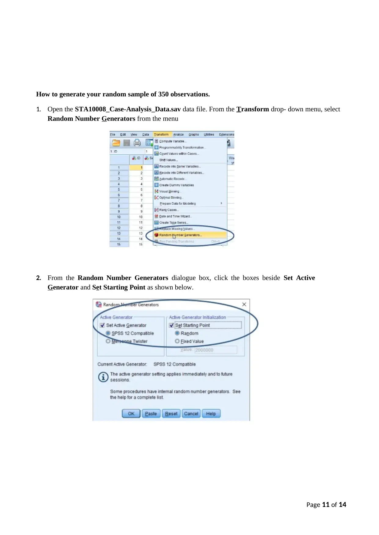
1. Open the STA10008_Case-Analysis_Data.sav data file. From the Transform drop- down menu, select
Random Number Generators from the menu
2. From the Random Number Generators dialogue box, click the boxes beside Set Active
Generator and Set Starting Point as shown below.
Page 11 of 14

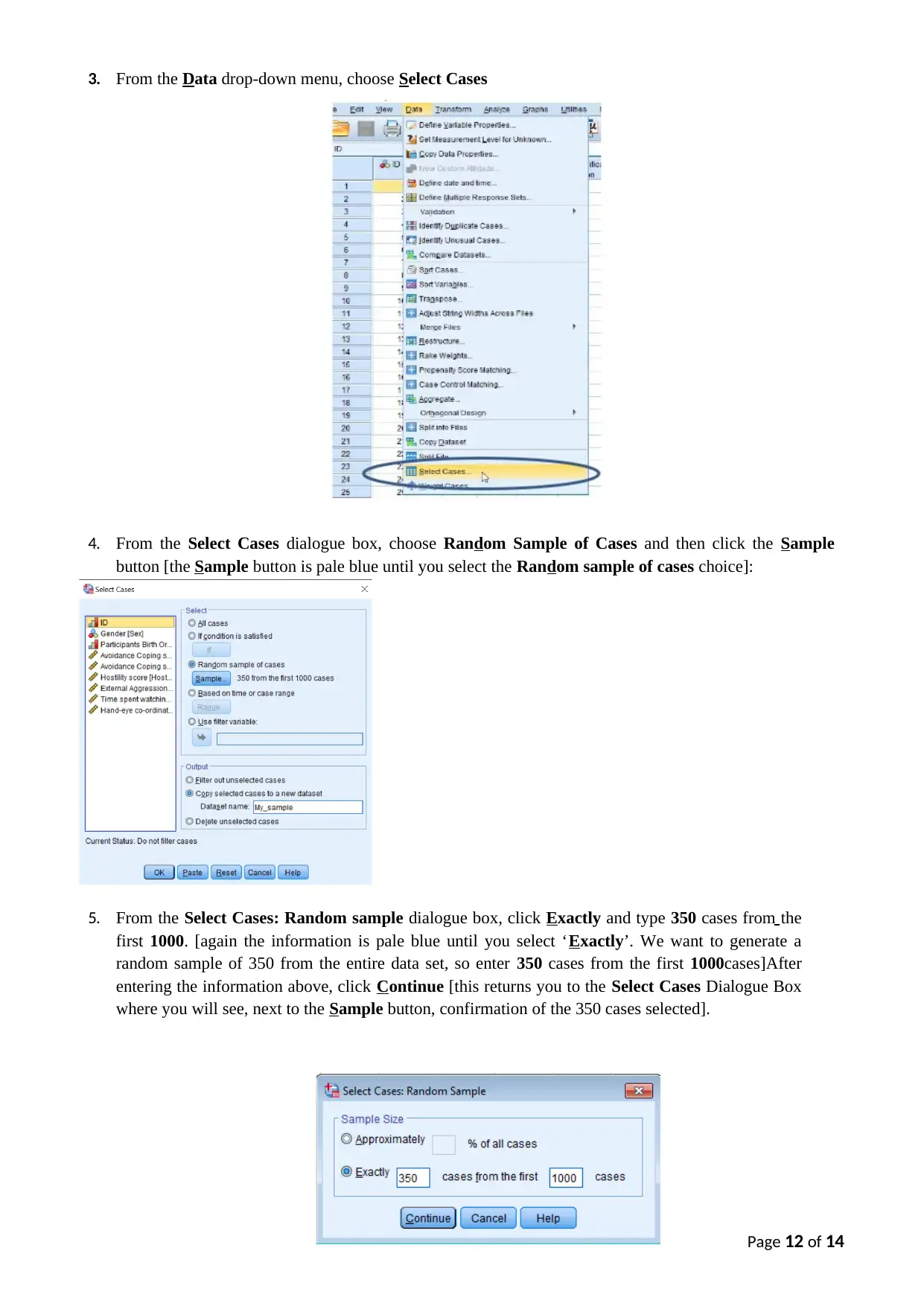
3. From the Data drop-down menu, choose Select Cases
4. From the Select Cases dialogue box, choose Random Sample of Cases and then click the Sample
button [the Sample button is pale blue until you select the Random sample of cases choice]:
5. From the Select Cases: Random sample dialogue box, click Exactly and type 350 cases from the
first 1000. [again the information is pale blue until you select ‘Exactly’. We want to generate a
random sample of 350 from the entire data set, so enter 350 cases from the first 1000cases]After
entering the information above, click Continue [this returns you to the Select Cases Dialogue Box
where you will see, next to the Sample button, confirmation of the 350 cases selected].
Page 12 of 14

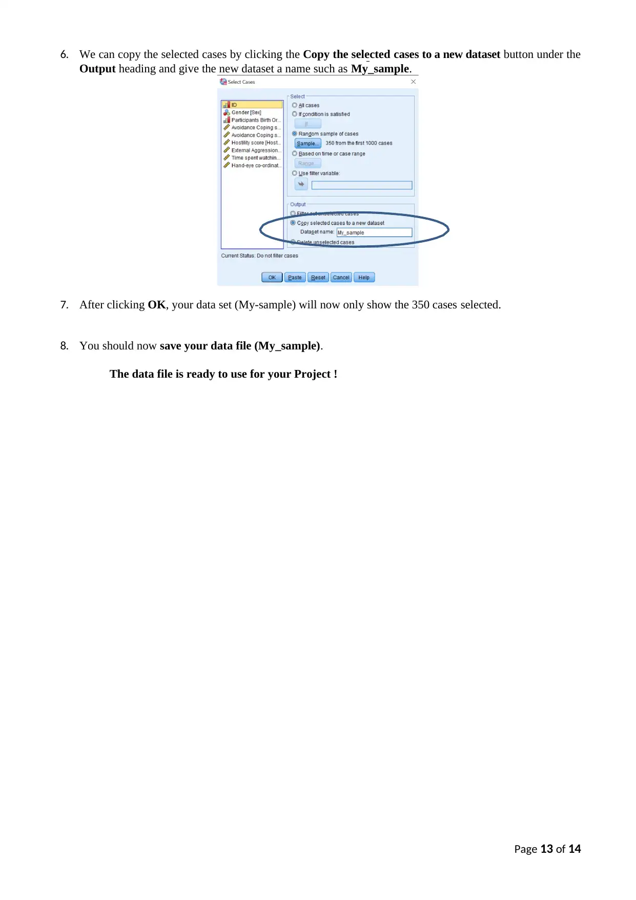
6. We can copy the selected cases by clicking the Copy the selected cases to a new dataset button under the
Output heading and give the new dataset a name such as My_sample.
7. After clicking OK, your data set (My-sample) will now only show the 350 cases selected.
8. You should now save your data file (My_sample).
The data file is ready to use for your Project !
Page 13 of 14

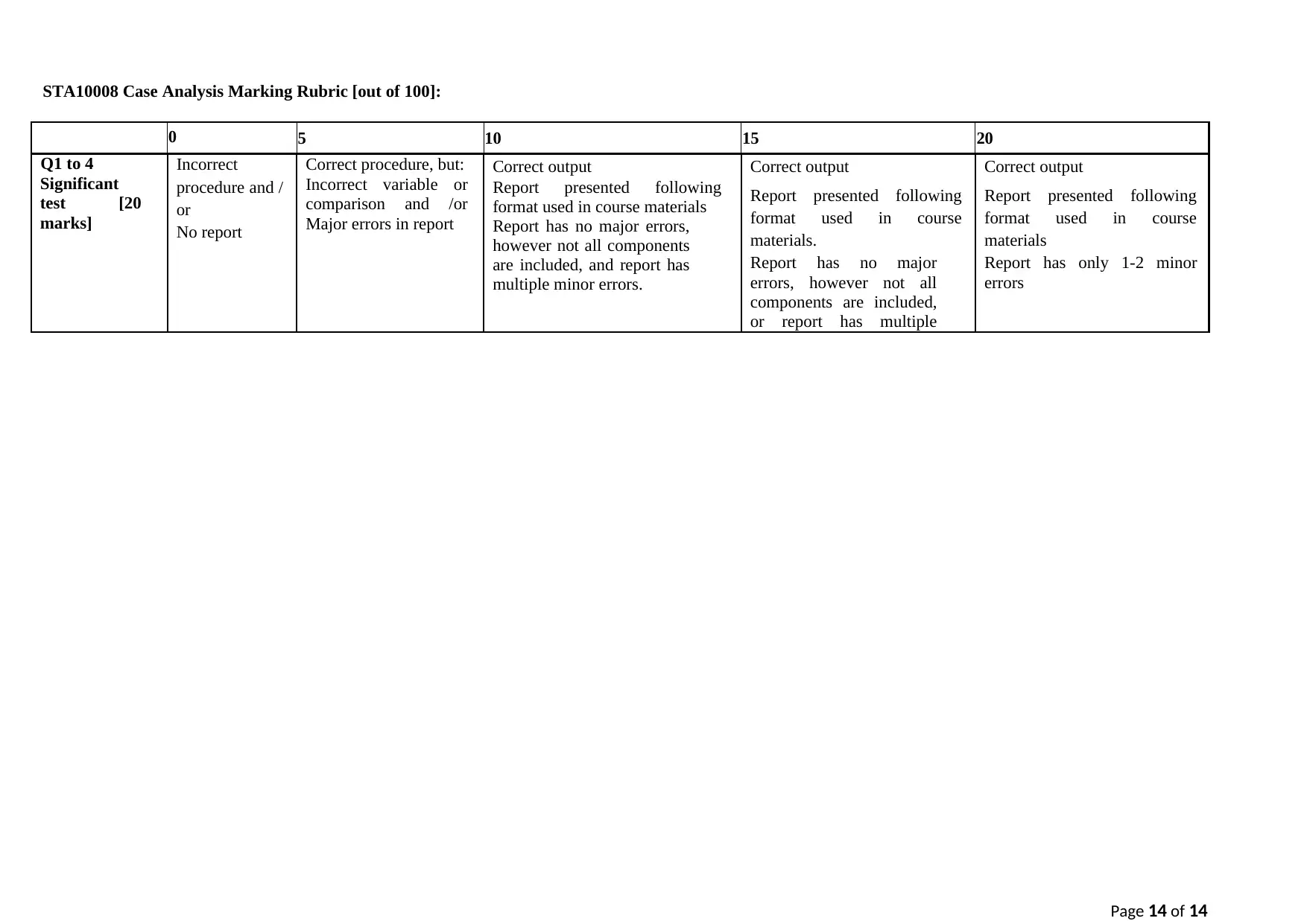
STA10008 Case Analysis Marking Rubric [out of 100]:
0 5 10 15 20
Q1 to 4
Significant
test [20
marks]
Incorrect
procedure and /
or
No report
Correct procedure, but:
Incorrect variable or
comparison and /or
Major errors in report
Correct output
Report presented following
format used in course materials
Report has no major errors,
however not all components
are included, and report has
multiple minor errors.
Correct output
Report presented following
format used in course
materials.
Report has no major
errors, however not all
components are included,
or report has multiple
minor errors.
Correct output
Report presented following
format used in course
materials
Report has only 1-2 minor
errors
Page 14 of 14