STA2300 Data Analysis S3, 18 Assignment 3 Solutions Due Date: 29 January, 2019
VerifiedAdded on 2023/04/22
|27
|5121
|151
AI Summary
Contribute Materials
Your contribution can guide someone’s learning journey. Share your
documents today.
STA2300 Data Analysis S3, 18
Assignment 3 Solutions
Due Date: 29 January, 2019
1
Assignment 3 Solutions
Due Date: 29 January, 2019
1
Secure Best Marks with AI Grader
Need help grading? Try our AI Grader for instant feedback on your assignments.
STA2300 Data Analysis S3, 18
Question 1
(a) 2 marks
Variable of interest: Number of swimmers (X) in Division A or the fastest division is
the variable of interest. We assume here that qualifying times for division A for each
swimmer is independent of others and have probability of (0.2) to qualify for the
aforesaid division.
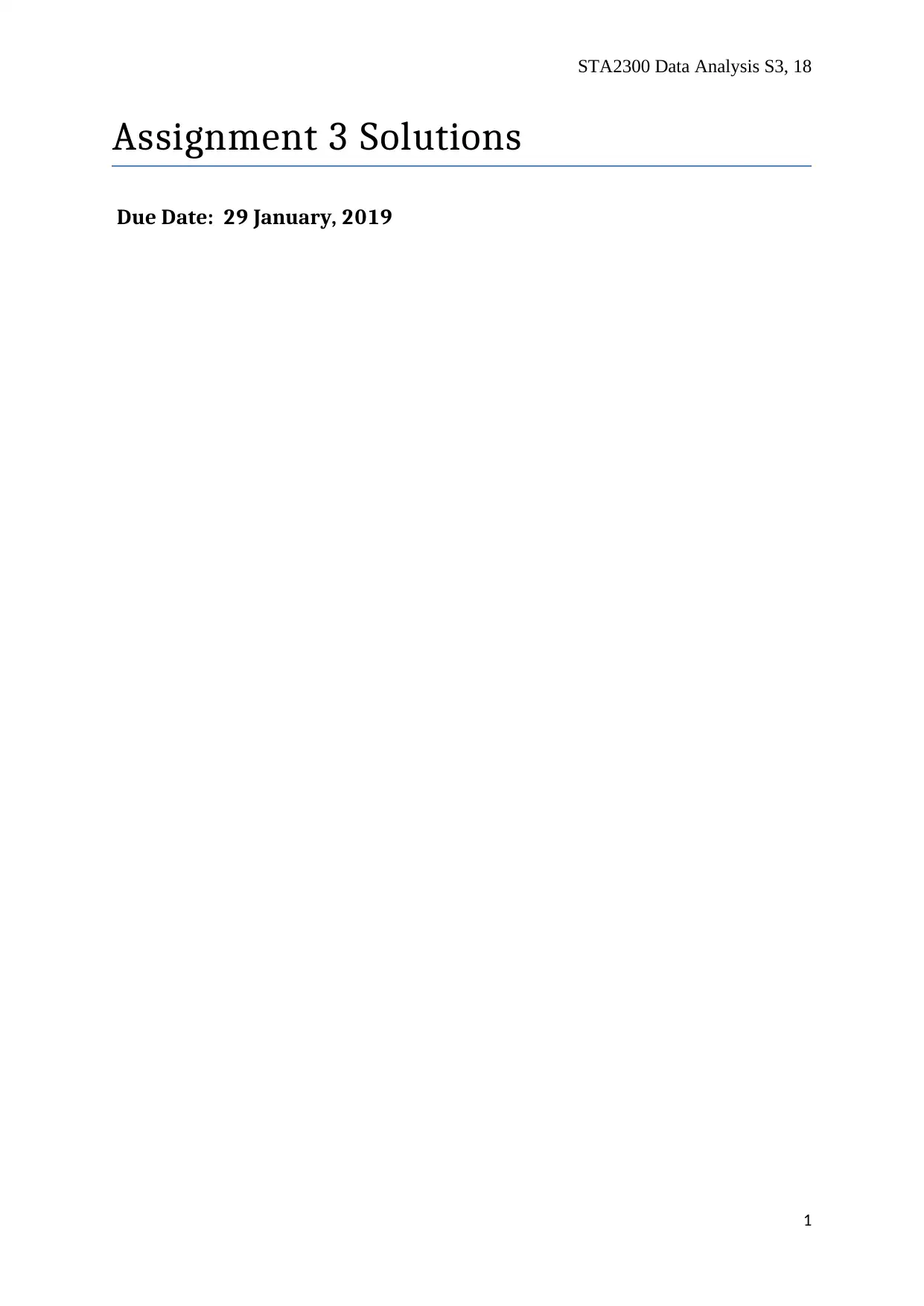
Sample Statistic: Amongst 186 total swimmers, 43 swimmers (23.1%) are in Division
A, 86 swimmers (46.2%) are in Division B, and 57 (30.6%) swimmers are in Division C.
Mean and Median for the division of the swimmers was Division B.
Figure 1: Percentage distribution of Swimmers in Divisions
(b) 3 marks
Hypotheses: Null hypothesis: H0: (p = 0.2) and the right tail Alternate hypothesis is HA:
( p>0 .2 )
Here, p denotes the probability that number of swimmers in Division A is 20% or 0.2.
The alternate hypothesis is in accordance with the researchers claim that number of
swimmers in Division A is more than 20%.
(c) 4 marks
Assumptions: The assumptions for one sample test of proportions are guided by
Binomial Model X ~ B ( n , p ) , where n = 186 is the number of swimmers and p = 0.2 is the
proportion or percentage f swimmers in Division A. Here the sample size was
considerably large ( n≥30 ) and therefore we will use normal approximation to binomial
model, by Central Limit Theorem (CLT).
2
Question 1
(a) 2 marks
Variable of interest: Number of swimmers (X) in Division A or the fastest division is
the variable of interest. We assume here that qualifying times for division A for each
swimmer is independent of others and have probability of (0.2) to qualify for the
aforesaid division.
Sample Statistic: Amongst 186 total swimmers, 43 swimmers (23.1%) are in Division
A, 86 swimmers (46.2%) are in Division B, and 57 (30.6%) swimmers are in Division C.
Mean and Median for the division of the swimmers was Division B.
Figure 1: Percentage distribution of Swimmers in Divisions
(b) 3 marks
Hypotheses: Null hypothesis: H0: (p = 0.2) and the right tail Alternate hypothesis is HA:
( p>0 .2 )
Here, p denotes the probability that number of swimmers in Division A is 20% or 0.2.
The alternate hypothesis is in accordance with the researchers claim that number of
swimmers in Division A is more than 20%.
(c) 4 marks
Assumptions: The assumptions for one sample test of proportions are guided by
Binomial Model X ~ B ( n , p ) , where n = 186 is the number of swimmers and p = 0.2 is the
proportion or percentage f swimmers in Division A. Here the sample size was
considerably large ( n≥30 ) and therefore we will use normal approximation to binomial
model, by Central Limit Theorem (CLT).
2
STA2300 Data Analysis S3, 18
Rule of Sample Proportions:
According to the said rule for sample proportions, np≥10 and n ( 1− p ) ≥10 should be
satisfied for the sampling distribution to be normally distributed.
Here, np=186∗0. 2=37. 2>10 and n ( 1− p ) =186∗0 . 8=148. 8>10 . Rule of sample
proportion is satisfied and the sampling distribution will have SE (standard error) of
√ p ( 1− p )
n = √ 0. 2∗0 .8
186 =0. 03 .
(d) 2 marks
The test statistic for one sample test of proportion is
Z = p
^¿ − p
√ p ( 1− p )
n
¿
where p
^¿
¿ is sample
proportion and p
^¿=43
186 =0 .23
¿ ,
Z = 0 . 23−0. 2
√ 0. 2∗0 .8
186
=1 .023
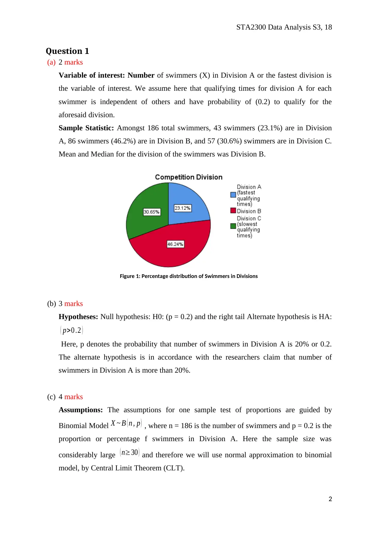
(e) 6 marks
Considering level of significance, α =0 . 05 for this right tail test, and using the Z-table we
get p=P ( Z >1 . 023 ) =0 . 1532> 0 .05 . As the p value is greater than level of significance,
the null hypothesis cannot be rejected at 5% level.
Figure 2: P-Value plot in Normal Curve
3
Rule of Sample Proportions:
According to the said rule for sample proportions, np≥10 and n ( 1− p ) ≥10 should be
satisfied for the sampling distribution to be normally distributed.
Here, np=186∗0. 2=37. 2>10 and n ( 1− p ) =186∗0 . 8=148. 8>10 . Rule of sample
proportion is satisfied and the sampling distribution will have SE (standard error) of
√ p ( 1− p )
n = √ 0. 2∗0 .8
186 =0. 03 .
(d) 2 marks
The test statistic for one sample test of proportion is
Z = p
^¿ − p
√ p ( 1− p )
n
¿
where p
^¿
¿ is sample
proportion and p
^¿=43
186 =0 .23
¿ ,
Z = 0 . 23−0. 2
√ 0. 2∗0 .8
186
=1 .023
(e) 6 marks
Considering level of significance, α =0 . 05 for this right tail test, and using the Z-table we
get p=P ( Z >1 . 023 ) =0 . 1532> 0 .05 . As the p value is greater than level of significance,
the null hypothesis cannot be rejected at 5% level.
Figure 2: P-Value plot in Normal Curve
3
STA2300 Data Analysis S3, 18
Therefore, we can conclude that there is not enough statistical evidence to support the
researcher’s belief that in recent year’s number of swimmers in Division A has grown
and surpassed the fastest 20% swimmers cut-off point. There is almost 15.32% chance
that fastest 20% swimmers are only in the Division A, and the probability is large enough
for not rejecting the null hypothesis.
(f) 4 marks
If Swimming Association wants to ensure that the margin error estimate of 99%
confidence is 0.02 of the actual proportion of senior swimmers in Group A, then the
minimum sample size is found as using a conservative method to determine sample size,
n= p
^¿∗¿ ¿
¿ ¿¿ Swimmers
(g) 3 marks
We get the required number of swimmers to ensure that the margin error estimate of 99%
confidence is 0.02 of the actual proportion of senior swimmers in Group A, using actual
proportion from the sample, then required sample size is,
n= p
^¿∗¿ ¿
¿ ¿¿ Swimmers
The impact of choosing the actual proportion from the sample is that number of
swimmers required will be considerable less, and this could result in less time and cost
for the research.
4
Secure Best Marks with AI Grader
Need help grading? Try our AI Grader for instant feedback on your assignments.
STA2300 Data Analysis S3, 18
Question 2
(a) 6 marks
Assumptions for Confidence Interval:
First, we assume that the swimmers are chosen randomly from the population of
swimmers. Secondly, number of the swimmers in Division-C are 57, which is greater
than 30. Hence, CLT can be applied on the distribution of the age of the swimmers to
establish that the data follows to a normal distribution. Third, it is also assumed that the
number of swimmers in Division-C is less than 10% of such swimmers in the population.
Assumptions for Hypothesis Testing:
The dependent variable, age of the swimmers in Division-C is continuous (interval/ratio).
The observations of age of the swimmers in Division-C are independent of one another.
The age of swimmers in Division-C, the dependent variable, is normally distributed. The
proof is accumulated from Shapiro-Wilk test for normality (W = 0.975, p = 0.275).
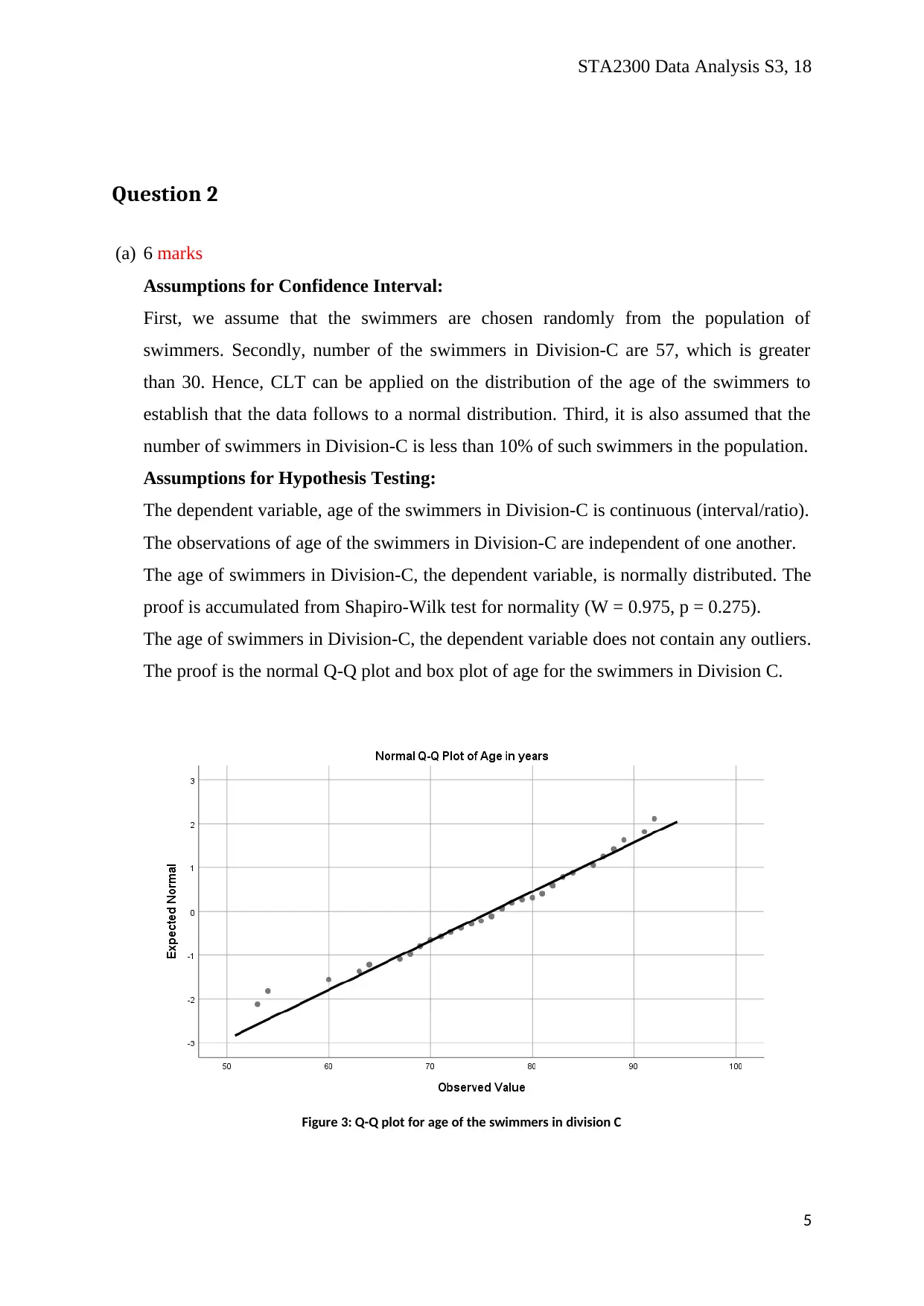
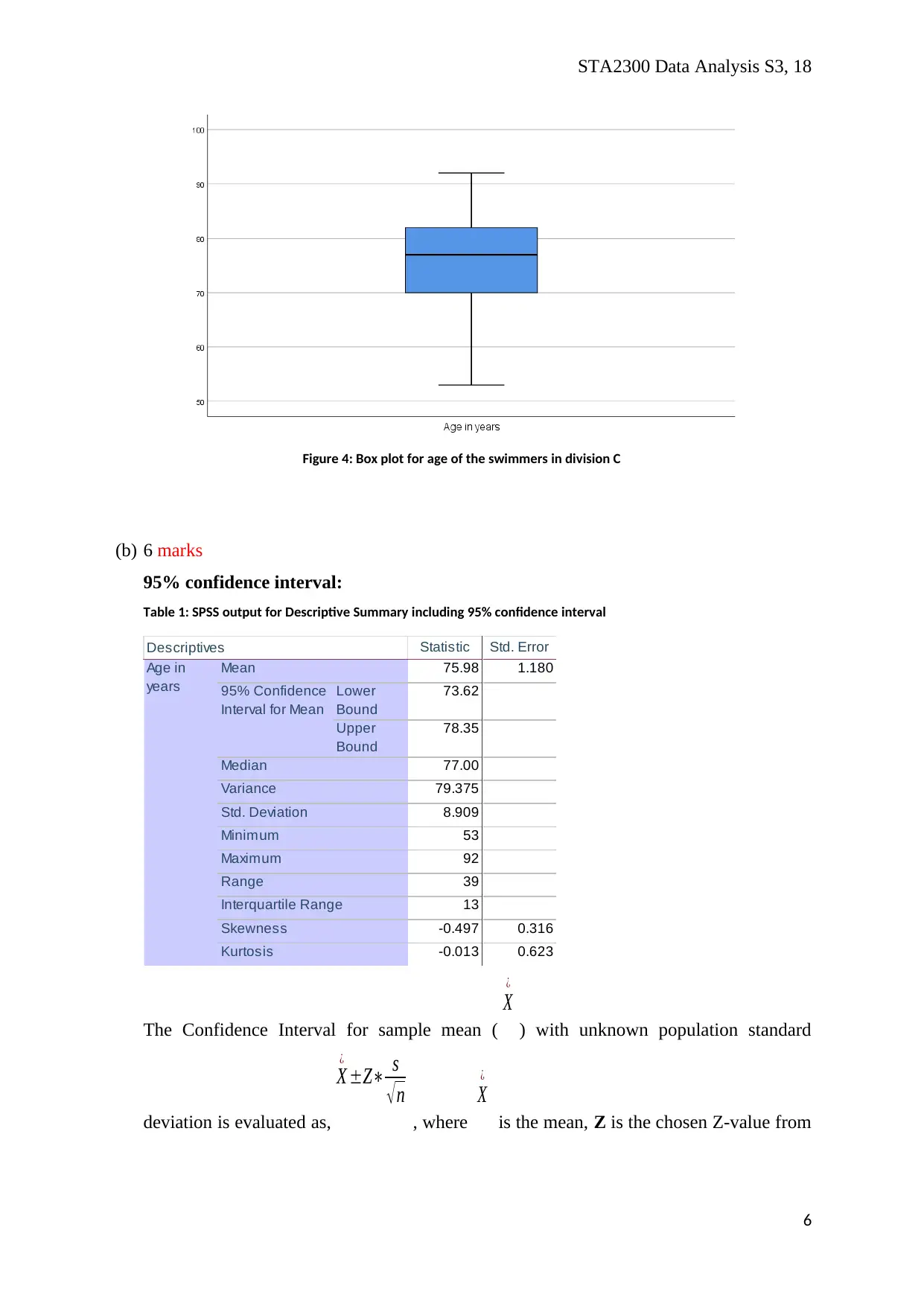
The age of swimmers in Division-C, the dependent variable does not contain any outliers.
The proof is the normal Q-Q plot and box plot of age for the swimmers in Division C.
Figure 3: Q-Q plot for age of the swimmers in division C
5
Question 2
(a) 6 marks
Assumptions for Confidence Interval:
First, we assume that the swimmers are chosen randomly from the population of
swimmers. Secondly, number of the swimmers in Division-C are 57, which is greater
than 30. Hence, CLT can be applied on the distribution of the age of the swimmers to
establish that the data follows to a normal distribution. Third, it is also assumed that the
number of swimmers in Division-C is less than 10% of such swimmers in the population.
Assumptions for Hypothesis Testing:
The dependent variable, age of the swimmers in Division-C is continuous (interval/ratio).
The observations of age of the swimmers in Division-C are independent of one another.
The age of swimmers in Division-C, the dependent variable, is normally distributed. The
proof is accumulated from Shapiro-Wilk test for normality (W = 0.975, p = 0.275).
The age of swimmers in Division-C, the dependent variable does not contain any outliers.
The proof is the normal Q-Q plot and box plot of age for the swimmers in Division C.
Figure 3: Q-Q plot for age of the swimmers in division C
5
STA2300 Data Analysis S3, 18
Figure 4: Box plot for age of the swimmers in division C
(b) 6 marks
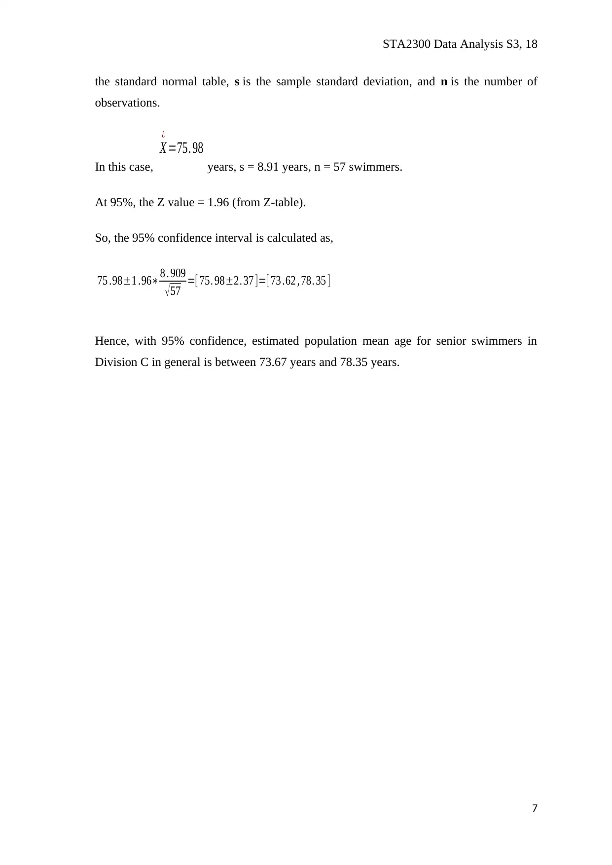
95% confidence interval:
Table 1: SPSS output for Descriptive Summary including 95% confidence interval
Statistic Std. Error
75.98 1.180
Lower
Bound
73.62
Upper
Bound
78.35
77.00
79.375
8.909
53
92
39
13
-0.497 0.316
-0.013 0.623
Maximum
Range
Interquartile Range
Skewness
Kurtosis
Descriptives
Age in
years
Mean
95% Confidence
Interval for Mean
Median
Variance
Std. Deviation
Minimum
The Confidence Interval for sample mean (
X
¿
) with unknown population standard
deviation is evaluated as,
X
¿
±Z∗ s
√ n
, where
X
¿
is the mean, Z is the chosen Z-value from
6
Figure 4: Box plot for age of the swimmers in division C
(b) 6 marks
95% confidence interval:
Table 1: SPSS output for Descriptive Summary including 95% confidence interval
Statistic Std. Error
75.98 1.180
Lower
Bound
73.62
Upper
Bound
78.35
77.00
79.375
8.909
53
92
39
13
-0.497 0.316
-0.013 0.623
Maximum
Range
Interquartile Range
Skewness
Kurtosis
Descriptives
Age in
years
Mean
95% Confidence
Interval for Mean
Median
Variance
Std. Deviation
Minimum
The Confidence Interval for sample mean (
X
¿
) with unknown population standard
deviation is evaluated as,
X
¿
±Z∗ s
√ n
, where
X
¿
is the mean, Z is the chosen Z-value from
6
STA2300 Data Analysis S3, 18
the standard normal table, s is the sample standard deviation, and n is the number of
observations.
In this case,
X
¿
=75. 98
years, s = 8.91 years, n = 57 swimmers.
At 95%, the Z value = 1.96 (from Z-table).
So, the 95% confidence interval is calculated as,
75 .98±1 .96∗8 . 909
√ 57 =[ 75. 98±2. 37 ]=[ 73 .62 , 78. 35 ]
Hence, with 95% confidence, estimated population mean age for senior swimmers in
Division C in general is between 73.67 years and 78.35 years.
7
Paraphrase This Document
Need a fresh take? Get an instant paraphrase of this document with our AI Paraphraser
STA2300 Data Analysis S3, 18
Question 3
(a) 3 marks
For the one sample test for mean, the Null hypothesis: H0:
( μ=80 )
(Assumes that
average age of senior swimmers in Division C is 80)
And the left tail alternate hypothesis is HA:
( μ<80 )
(Assumes that average age of senior
swimmers in Division C in accordance to the researcher is less than 80), where
( μ )
is the
average age of senior swimmers in Division C.
(b) 2 marks
The sample size n = 57 is greater than 30, hence the sampling distribution of age of the
swimmers in Division C is considered to be normally distributed. The test statistic for
one sample test for mean is
t = x
¿
−μ
s / √ n with n-1 degrees of freedom. x
−
: The sample mean,
s: the sample standard deviation, and n is the sample size.
Average age of the swimmers in Division C is x
−
=75 . 98 years, standard deviation of age
in sample is s = 8.91 years, n = 57 swimmers in Division C.
Hence,
t= x
¿
−μ
s / √ n =75. 98−80
8. 91/ √ 57 =−4 . 02
1. 18 =−3 . 41 the value of the test statistic for one sample
test for mean
(c) 6 marks
Considering level of significance, α=0 . 05 for this right left test, and using the t-table we
get p=P ( t ( 56)<−3 . 41 ) =0 .0006 <0 .05 . As the p value is less than level of significance,
the null hypothesis can be rejected at 5% level.
8
STA2300 Data Analysis S3, 18
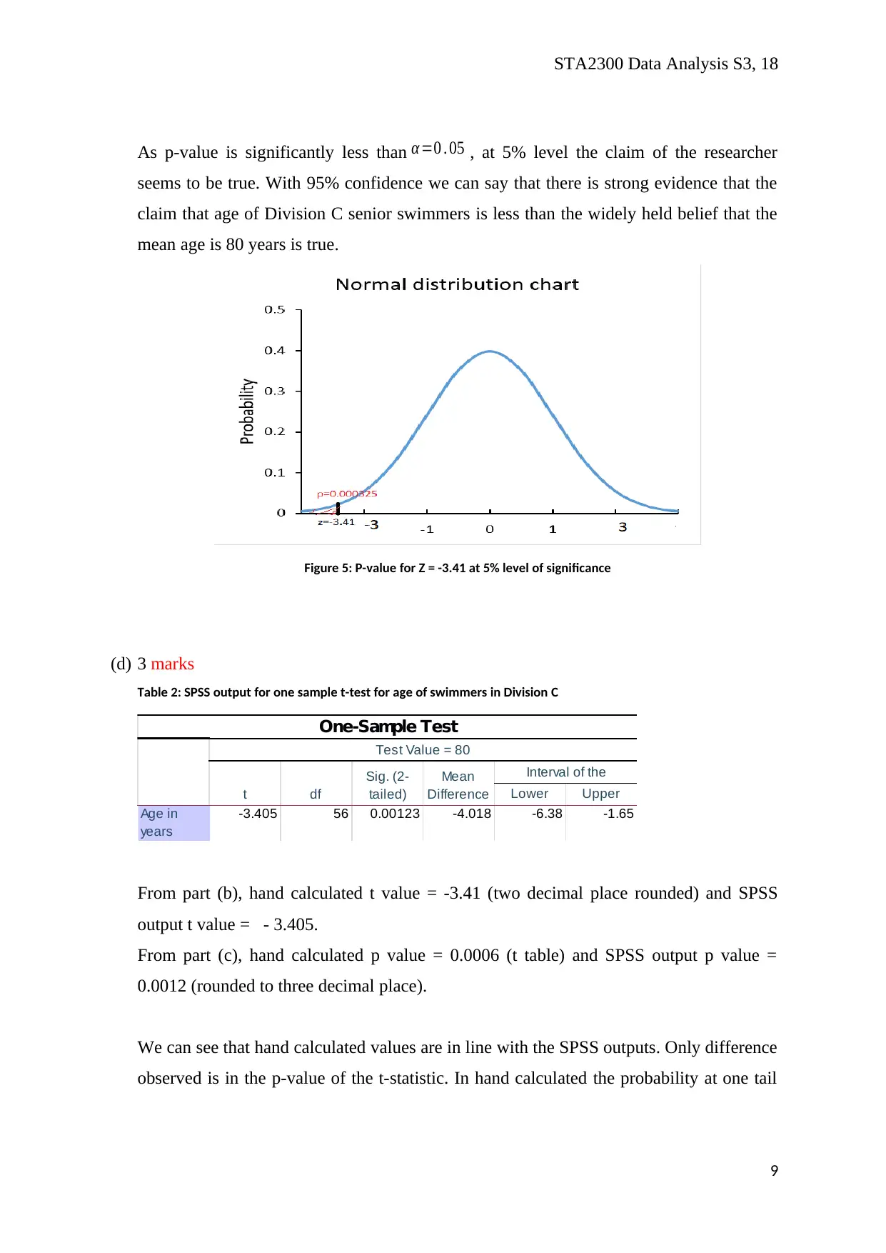
As p-value is significantly less than α=0 . 05 , at 5% level the claim of the researcher
seems to be true. With 95% confidence we can say that there is strong evidence that the
claim that age of Division C senior swimmers is less than the widely held belief that the
mean age is 80 years is true.
Figure 5: P-value for Z = -3.41 at 5% level of significance
(d) 3 marks
Table 2: SPSS output for one sample t-test for age of swimmers in Division C
Lower Upper
Age in
years
-3.405 56 0.00123 -4.018 -6.38 -1.65
95% Confidence
Interval of the
One-Sample Test
Test Value = 80
t df
Sig. (2-
tailed)
Mean
Difference
From part (b), hand calculated t value = -3.41 (two decimal place rounded) and SPSS
output t value = - 3.405.
From part (c), hand calculated p value = 0.0006 (t table) and SPSS output p value =
0.0012 (rounded to three decimal place).
We can see that hand calculated values are in line with the SPSS outputs. Only difference
observed is in the p-value of the t-statistic. In hand calculated the probability at one tail
9
STA2300 Data Analysis S3, 18
has been calculated, whereas, the p-value in the SPSS output is for two tail. Therefore,
the SPSS p-value is double the p-value calculated by hand.
Question 4
(a) 4 marks
Figure 6: Boxplot for Competition time for swimmers in the 50-59 and 60-69 year age group
(b) 2 marks
Median time taken for competition in age group of 50-59 years is below 400 seconds
(Median = 370 seconds: from SPSS output). The median time taken for competition in
age group of 60-69 years is above 400 seconds (Median = 449 seconds: from SPSS
output). Therefore, it is noted that swimmers in 50-59 age group are faster than
swimmers of 60-69 age group. Two outliers for competition timing for each age group
are noted from the boxplot in Figure 5. The spread of competition timing of 60-69 age
group is considerably higher (R = 292 – 1071 seconds) than competition timing of age
group 50-59 (R = 305 - 580 seconds). This implied that swimmers in age group 50-59
10
Secure Best Marks with AI Grader
Need help grading? Try our AI Grader for instant feedback on your assignments.
STA2300 Data Analysis S3, 18
have less difference in competition time amongst them compared to that of the swimmers
of age group 60-69.
(c) 5 marks
To test whether senior swimmers in the 50-59 year age group swim faster than swimmers
in the 60-69 year group, average competition times of the two age groups are compared.
Null hypothesis: H0: ( μ1=μ2 ) where ( μ1 ) is the average competition time taken by
swimmers in age group 50-59, and ( μ2 ) is the average competition time taken by
swimmers in age group 60-69.
Alternate hypothesis: H0: ( μ1< μ2 ) (where the researcher thinks swimmers in 50-59
perform better than 60-69 age group).
The appropriate test to check the scenario is independent t-test.
Assumptions of independent t-test are:
Independent observations: The competition times from each age group are of different
participants, and seem to be independent in our data. .
Normality: The dependent variable is the competition time of the swimmers. There are
107 swimmers in the two age groups (50-59, 60-69). From Shapiro-Wilk test in SPSS we
get that competition time is significantly (W = 0.83, p < 0.05) not normal. This is because
of the outlier observations in the swimming time. But, due to sample size of 107 (n > 30)
the sampling distribution is considered to follow from CLT (Central Limit Theorem).
Homogeneity: The standard deviations of competition time for the two groups are
compared by Levene’s test (F = 4.88, p = 0.029), and at 5% level of significance the
standard deviations of competition time of the two groups are found to be unequal.
(d) 2 marks
The test statistic is calculated as,
t= x1−x2
√ s1
2
n1
+ s2
2
n2
Now, for competition time of the age group 50-59,
x
−
1=15346
40 =383 . 65 , s1= √ ∑ ( xi−x
−
)
2
n1
= √ 180198 . 406
40 =67 . 12, n1=40
And for competition time of the age group 60-69,
11
STA2300 Data Analysis S3, 18
x
−
2=31169. 07
67 =465 . 21 , s2= √ ∑ ( xi−x
−
)
2
n2
= √ 1001286 . 42
67 =122. 25 , n2=67
Hence,
t= x1−x2
√ s1
2
n1
+ s2
2
n2
=383 .65−465 . 21
√ 67 . 122
40 +122 . 252
67
=−3 . 88
(two decimal places) for (40 + 67 – 2)
= 105 degrees of freedom.
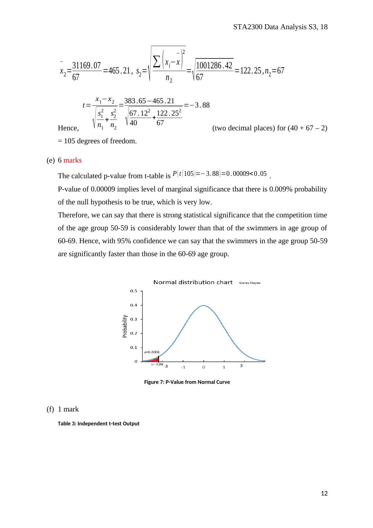
(e) 6 marks
The calculated p-value from t-table is P ( t ( 105 ) =−3. 88 ) =0 . 00009< 0 .05 .
P-value of 0.00009 implies level of marginal significance that there is 0.009% probability
of the null hypothesis to be true, which is very low.
Therefore, we can say that there is strong statistical significance that the competition time
of the age group 50-59 is considerably lower than that of the swimmers in age group of
60-69. Hence, with 95% confidence we can say that the swimmers in the age group 50-59
are significantly faster than those in the 60-69 age group.
Figure 7: P-Value from Normal Curve
(f) 1 mark
Table 3: Independent t-test Output
12
x
−
2=31169. 07
67 =465 . 21 , s2= √ ∑ ( xi−x
−
)
2
n2
= √ 1001286 . 42
67 =122. 25 , n2=67
Hence,
t= x1−x2
√ s1
2
n1
+ s2
2
n2
=383 .65−465 . 21
√ 67 . 122
40 +122 . 252
67
=−3 . 88
(two decimal places) for (40 + 67 – 2)
= 105 degrees of freedom.
(e) 6 marks
The calculated p-value from t-table is P ( t ( 105 ) =−3. 88 ) =0 . 00009< 0 .05 .
P-value of 0.00009 implies level of marginal significance that there is 0.009% probability
of the null hypothesis to be true, which is very low.
Therefore, we can say that there is strong statistical significance that the competition time
of the age group 50-59 is considerably lower than that of the swimmers in age group of
60-69. Hence, with 95% confidence we can say that the swimmers in the age group 50-59
are significantly faster than those in the 60-69 age group.
Figure 7: P-Value from Normal Curve
(f) 1 mark
Table 3: Independent t-test Output
12
STA2300 Data Analysis S3, 18
Lower Upper
Equal
variances
assumed
4.886 0.029 -3.880 105 0.000 -81.559 21.020 -123.238 -39.880
Equal
variances
not
assumed
-4.452 104.423 0.000 -81.559 18.321 -117.889 -45.229
Mean
Difference
Std. Error
Difference
95% Confidence
Interval of the
Competiti
on Time
Independent Samples Test (Gary Hayes)Levene's Test for
Equality of Variances t-test for Equality of Means
F Sig. t df
Sig. (2-
tailed)
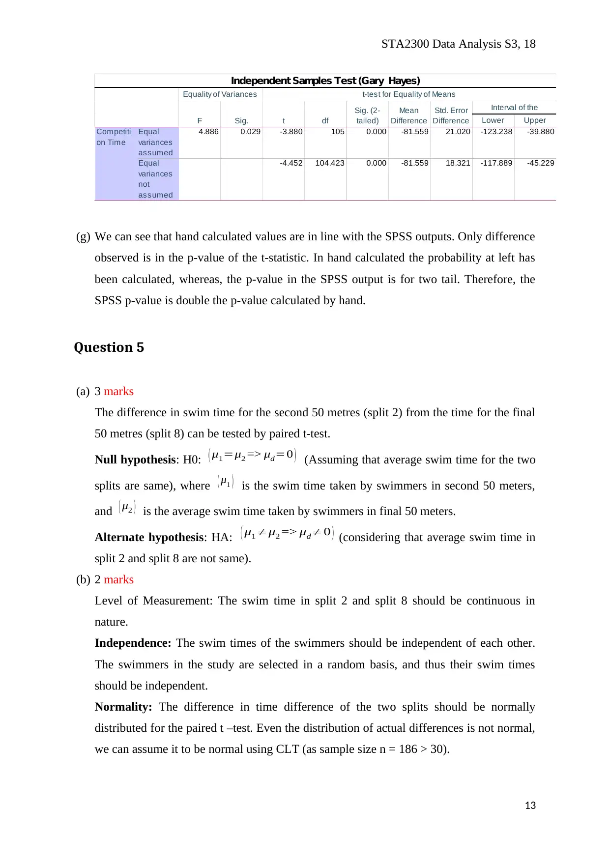
(g) We can see that hand calculated values are in line with the SPSS outputs. Only difference
observed is in the p-value of the t-statistic. In hand calculated the probability at left has
been calculated, whereas, the p-value in the SPSS output is for two tail. Therefore, the
SPSS p-value is double the p-value calculated by hand.
Question 5
(a) 3 marks
The difference in swim time for the second 50 metres (split 2) from the time for the final
50 metres (split 8) can be tested by paired t-test.
Null hypothesis: H0: ( μ1=μ2 => μd=0 ) (Assuming that average swim time for the two
splits are same), where ( μ1 ) is the swim time taken by swimmers in second 50 meters,
and ( μ2 ) is the average swim time taken by swimmers in final 50 meters.
Alternate hypothesis: HA: ( μ1≠μ2 => μd≠0 ) (considering that average swim time in
split 2 and split 8 are not same).
(b) 2 marks
Level of Measurement: The swim time in split 2 and split 8 should be continuous in
nature.
Independence: The swim times of the swimmers should be independent of each other.
The swimmers in the study are selected in a random basis, and thus their swim times
should be independent.
Normality: The difference in time difference of the two splits should be normally
distributed for the paired t –test. Even the distribution of actual differences is not normal,
we can assume it to be normal using CLT (as sample size n = 186 > 30).
13
Lower Upper
Equal
variances
assumed
4.886 0.029 -3.880 105 0.000 -81.559 21.020 -123.238 -39.880
Equal
variances
not
assumed
-4.452 104.423 0.000 -81.559 18.321 -117.889 -45.229
Mean
Difference
Std. Error
Difference
95% Confidence
Interval of the
Competiti
on Time
Independent Samples Test (Gary Hayes)Levene's Test for
Equality of Variances t-test for Equality of Means
F Sig. t df
Sig. (2-
tailed)
(g) We can see that hand calculated values are in line with the SPSS outputs. Only difference
observed is in the p-value of the t-statistic. In hand calculated the probability at left has
been calculated, whereas, the p-value in the SPSS output is for two tail. Therefore, the
SPSS p-value is double the p-value calculated by hand.
Question 5
(a) 3 marks
The difference in swim time for the second 50 metres (split 2) from the time for the final
50 metres (split 8) can be tested by paired t-test.
Null hypothesis: H0: ( μ1=μ2 => μd=0 ) (Assuming that average swim time for the two
splits are same), where ( μ1 ) is the swim time taken by swimmers in second 50 meters,
and ( μ2 ) is the average swim time taken by swimmers in final 50 meters.
Alternate hypothesis: HA: ( μ1≠μ2 => μd≠0 ) (considering that average swim time in
split 2 and split 8 are not same).
(b) 2 marks
Level of Measurement: The swim time in split 2 and split 8 should be continuous in
nature.
Independence: The swim times of the swimmers should be independent of each other.
The swimmers in the study are selected in a random basis, and thus their swim times
should be independent.
Normality: The difference in time difference of the two splits should be normally
distributed for the paired t –test. Even the distribution of actual differences is not normal,
we can assume it to be normal using CLT (as sample size n = 186 > 30).
13
Paraphrase This Document
Need a fresh take? Get an instant paraphrase of this document with our AI Paraphraser
STA2300 Data Analysis S3, 18
Outliers: There should not be any outlier swimming time so that the difference in split
times produces unusual or out of the box values. Presences of outliers provide incorrect
value of the statistic and conclusion from the test gets affected.
(c) 2 marks
Suitable test statistic for paired t-test is
t= x
−
1−x
−
2
SE ( d
−
) where ( x
−
1 ) is the average swim time
taken by 186 swimmers in second 50 meters, and ( x2 )
−
is the average swim time taken by
186 swimmers in final 50 meters, and SE ( d
−
) is the standard error of the differences
between the swim times of the two splits.
Now x
−
1=11457. 34
186 =62 .19 ,
x
−
2=11481. 73
186 =61. 73 , and
SE ( d
−
) = sd (d
−
)
√ n = 3 .545
√ 187 =0 .2592
So the test statistic is
t = x
−
1−x
−
2
SE ( d
−
) =62 .19−61. 73
0 . 2592 =1. 7747
(Please see Appendix for
detailed table of calculation)
(d) 6 marks
The p-value is calculated from the t-test statistic using t-table as,
P ( |t ( 185 ) |>1 .7747 ) =0 . 0776 > 0.05 at 5% level of significance.
P-value of 0.0776 implies level of marginal significance that there is 7.76% probability
of the null hypothesis to be true, which is quite acceptable.
14
STA2300 Data Analysis S3, 18
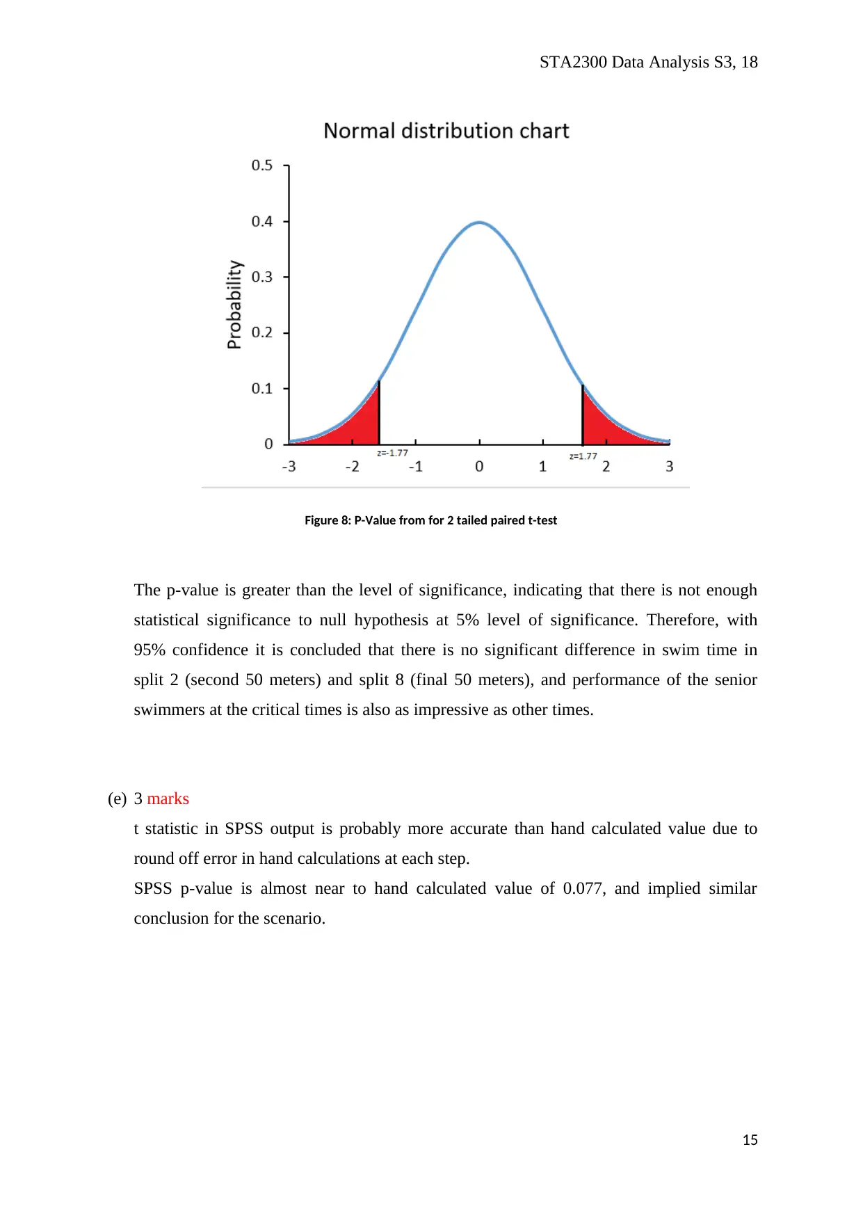
Figure 8: P-Value from for 2 tailed paired t-test
The p-value is greater than the level of significance, indicating that there is not enough
statistical significance to null hypothesis at 5% level of significance. Therefore, with
95% confidence it is concluded that there is no significant difference in swim time in
split 2 (second 50 meters) and split 8 (final 50 meters), and performance of the senior
swimmers at the critical times is also as impressive as other times.
(e) 3 marks
t statistic in SPSS output is probably more accurate than hand calculated value due to
round off error in hand calculations at each step.
SPSS p-value is almost near to hand calculated value of 0.077, and implied similar
conclusion for the scenario.
15
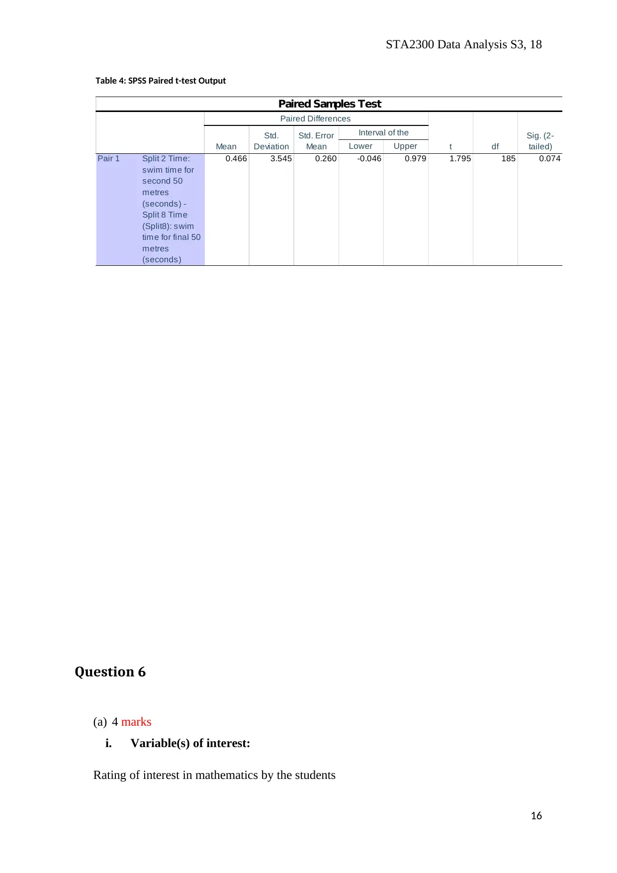
STA2300 Data Analysis S3, 18
Table 4: SPSS Paired t-test Output
Lower Upper
Pair 1 Split 2 Time:
swim time for
second 50
metres
(seconds) -
Split 8 Time
(Split8): swim
time for final 50
metres
(seconds)
0.466 3.545 0.260 -0.046 0.979 1.795 185 0.074
Paired Samples Test
Paired Differences
t df
Sig. (2-
tailed)Mean
Std.
Deviation
Std. Error
Mean
95% Confidence
Interval of the
Question 6
(a) 4 marks
i. Variable(s) of interest:
Rating of interest in mathematics by the students
16
Secure Best Marks with AI Grader
Need help grading? Try our AI Grader for instant feedback on your assignments.
STA2300 Data Analysis S3, 18
ii. Appropriate statistical method:
Paired t-test is the appropriate test statistic.
iii. Definition of the test statistic: The statistic
t= x
−
1−x
−
2
SE ( d
−
) ( x
−
1 ) is the average
interest rate by 9 children before watching television program, and ( x2 )
−
is the
average interest rate by 9 children after watching television program, and SE ( d
−
) is
the standard error of the differences between the interest rates of the two
situations.
iv. The null and alternative hypotheses:
Null hypothesis: There is no difference in average scores for interest in mathematics
before and after watching a new television program: H0: ( μ1=μ2 => μd=0 )
Alternate hypothesis: There is significant difference in average scores for interest in
mathematics before and after watching a new television program: HA:
( μ1≠μ2 => μd≠0 )
v. Conclusion:
Test statistic t (8) = 6, p = 0.289 > 0.05 imply that there is no significant difference in
average scores for interest in mathematics before and after watching a new television
program. Hence, there is no significant impact of the new television program.
(b) 4 marks
i. Variable(s) of interest:
Bus drivers stay time on the task
ii. Appropriate statistical method
17
STA2300 Data Analysis S3, 18
Paired t-test is the appropriate test statistic (Kim 2015, p.540-546).
iii. Definition of the test statistic
The statistic
t= x
−
1−x
−
2
SE ( d
−
) ( x
−
1 ) is the average stay time on the task of 25 bus drivers
before taking alcohol and ( x2 )
−
is the average stay time on the task of 25 bus drivers
after taking alcohol, and SE ( d
−
) is the standard error of the differences between the
stay times of the two situations.
iv. The null and alternative hypotheses
Null hypothesis: There is no difference in average stay time on the task before and
after consuming alcohol: H0: ( μ1=μ2 => μd=0 )
Alternate hypothesis: There is significant difference in average stay time on the task
before and after consuming alcohol: HA: ( μ1≠μ2 => μd≠0 )
v. Conclusion
Test statistic t (24) = 2, p = 0.057 > 0.05 imply that there is no significant difference
in average stay time on the task before and after consuming alcohol for the drivers.
Hence, there is no significant impact of alcohol on the drivers at 5% level of
significance. But, at 90% confidence level p-value = 0.057 < 0.01 implies that alcohol
has a deterrent impact on the drivers.
(c) 4 marks
i. Variable(s) of interest
Overall time of exercising and gender of the participants are the variable of interest.
18
STA2300 Data Analysis S3, 18
ii. Appropriate statistical method
Independent sample t-test is the appropriate test statistic (Park 2004, p.2017).
iii. Definition of the test statistic
The statistic
t = x1−x2
√ s1
2
n1
+ s2
2
n2 , where ( x
−
1 ) is the average time of exercising of males and
( x2 )
−
is the average time of exercising of females
s1 , s1 are the standard deviations of the time of exercising of males and females.
n1 , n2 are the sample size of the males and females.
iv. The null and alternative hypotheses
Null hypothesis: There is no difference in average time of exercising of males and
females: H0: ( μ1=μ2 )
Alternate hypothesis: There is significant difference in average time of exercising of
males and females: HA: ( μ1≠μ2 )
v. Conclusion
Test statistic t = 2.38, p = 0.016 < 0.05 imply that there is significant difference in
average time of exercising of males and females at 5% level of significance. But, at
99% confidence level, p-value = 0.016 > 0.01 implies that there is no significant
difference in average time of exercising of males and females.
References
19
Paraphrase This Document
Need a fresh take? Get an instant paraphrase of this document with our AI Paraphraser
STA2300 Data Analysis S3, 18
Kim, T.K., 2015. T test as a parametric statistic. Korean journal of anesthesiology, 68(6),
pp.540-546.
Park, H.M., 2004. Understanding the statistical power of a test. Retrieved April, 8, p.2017.
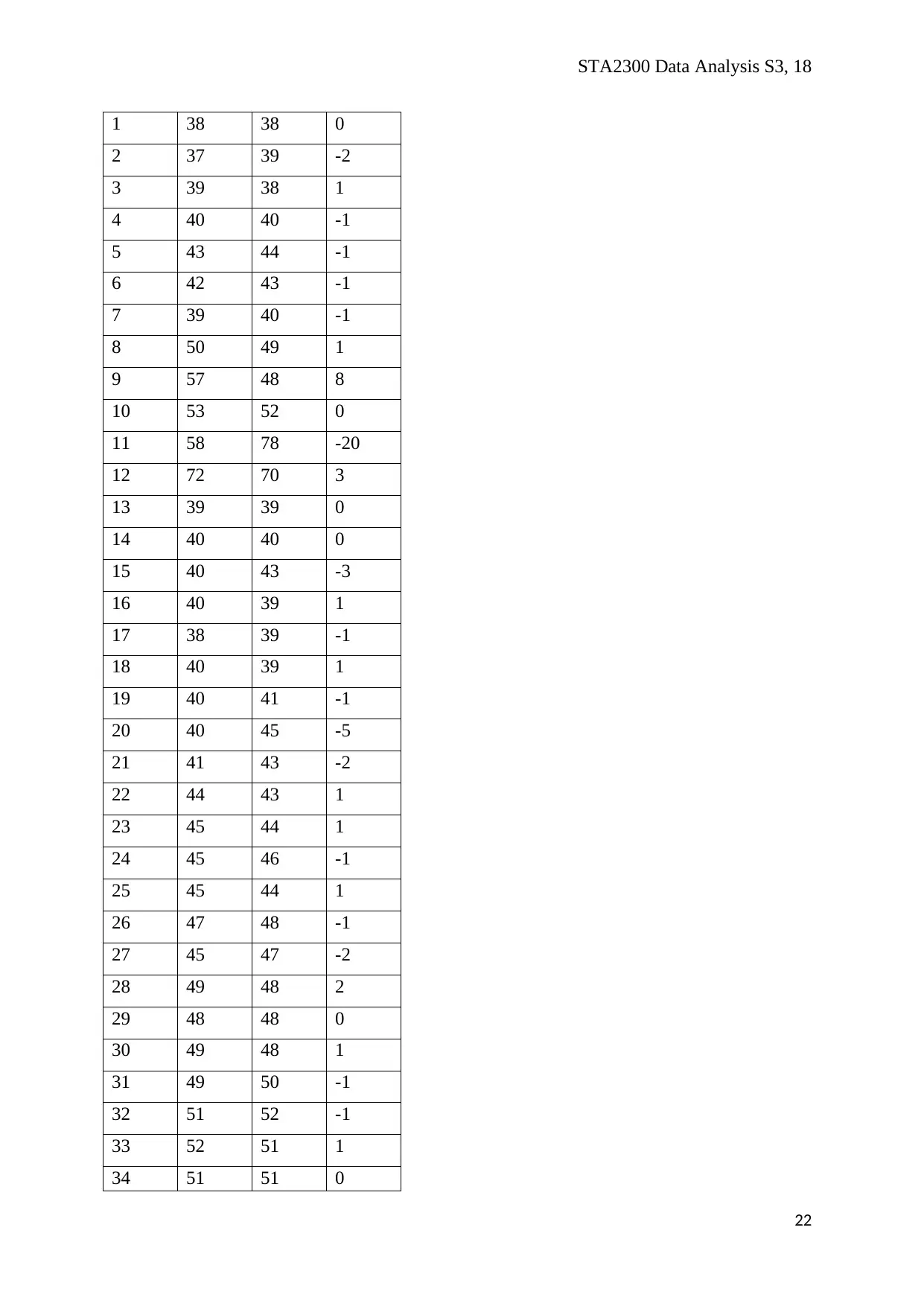
Appendices (Question 5)
20
Kim, T.K., 2015. T test as a parametric statistic. Korean journal of anesthesiology, 68(6),
pp.540-546.
Park, H.M., 2004. Understanding the statistical power of a test. Retrieved April, 8, p.2017.
Appendices (Question 5)
20
STA2300 Data Analysis S3, 18
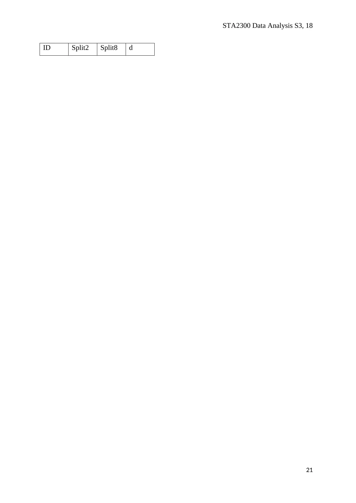
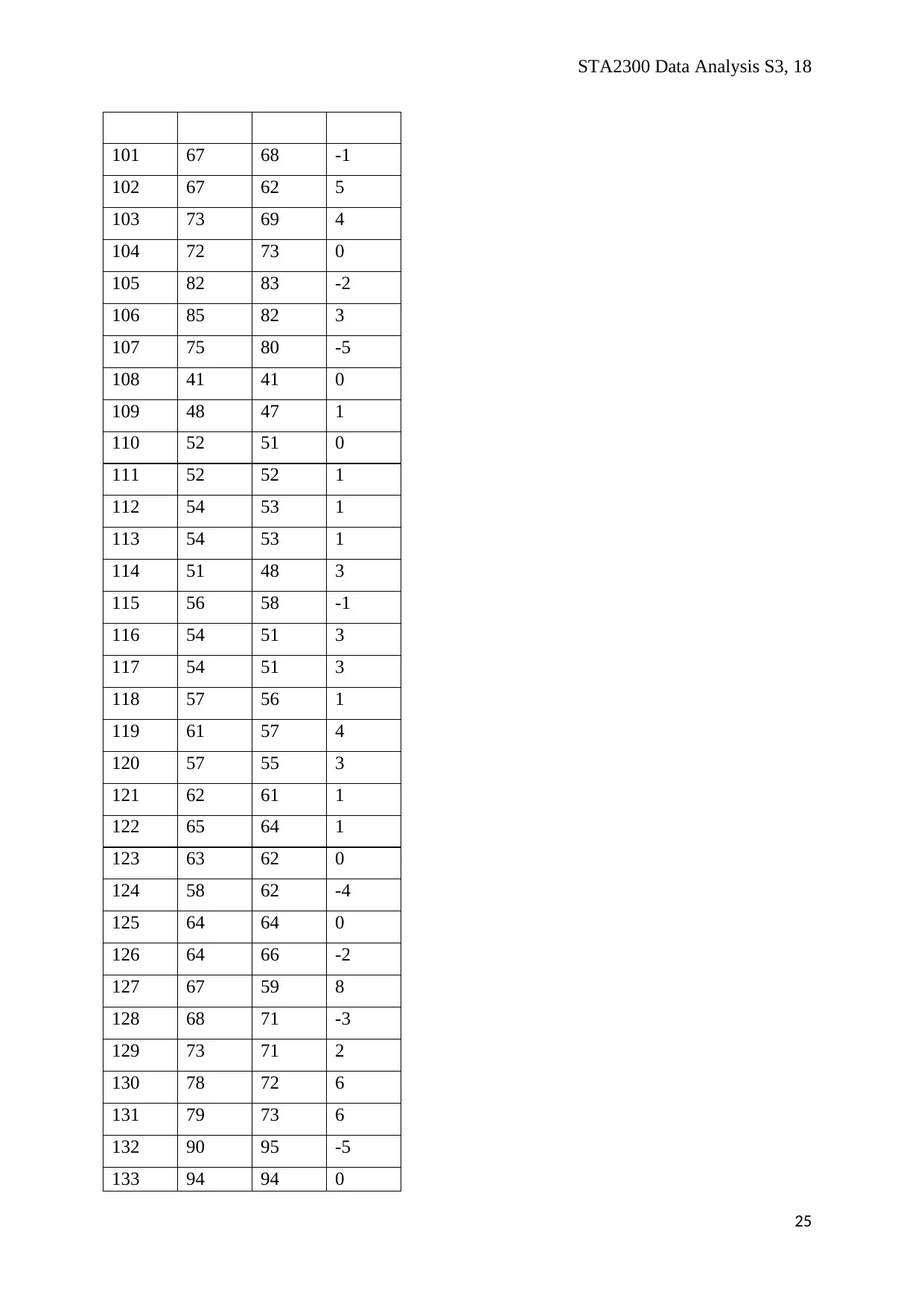
ID Split2 Split8 d
21
ID Split2 Split8 d
21
STA2300 Data Analysis S3, 18
1 38 38 0
2 37 39 -2
3 39 38 1
4 40 40 -1
5 43 44 -1
6 42 43 -1
7 39 40 -1
8 50 49 1
9 57 48 8
10 53 52 0
11 58 78 -20
12 72 70 3
13 39 39 0
14 40 40 0
15 40 43 -3
16 40 39 1
17 38 39 -1
18 40 39 1
19 40 41 -1
20 40 45 -5
21 41 43 -2
22 44 43 1
23 45 44 1
24 45 46 -1
25 45 44 1
26 47 48 -1
27 45 47 -2
28 49 48 2
29 48 48 0
30 49 48 1
31 49 50 -1
32 51 52 -1
33 52 51 1
34 51 51 0
22
Secure Best Marks with AI Grader
Need help grading? Try our AI Grader for instant feedback on your assignments.
STA2300 Data Analysis S3, 18
35 51 55 -4
36 56 54 2
37 58 57 1
38 58 60 -1
39 50 47 3
40 61 61 1
41 36 36 0
42 39 40 -1
43 41 42 -1
44 40 41 -1
45 45 45 -1
46 44 43 0
47 40 39 1
48 45 46 0
49 49 48 1
50 45 45 -1
51 48 47 1
52 48 48 0
53 46 45 1
54 46 46 0
55 48 48 0
56 49 47 2
57 49 49 -1
58 55 59 -5
59 53 50 2
60 50 55 -5
61 56 58 -1
62 58 51 8
63 55 56 0
64 52 51 1
65 59 56 2
66 59 60 -1
67 52 50 1
23
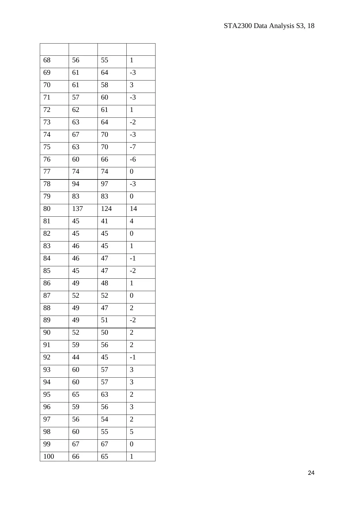
STA2300 Data Analysis S3, 18
68 56 55 1
69 61 64 -3
70 61 58 3
71 57 60 -3
72 62 61 1
73 63 64 -2
74 67 70 -3
75 63 70 -7
76 60 66 -6
77 74 74 0
78 94 97 -3
79 83 83 0
80 137 124 14
81 45 41 4
82 45 45 0
83 46 45 1
84 46 47 -1
85 45 47 -2
86 49 48 1
87 52 52 0
88 49 47 2
89 49 51 -2
90 52 50 2
91 59 56 2
92 44 45 -1
93 60 57 3
94 60 57 3
95 65 63 2
96 59 56 3
97 56 54 2
98 60 55 5
99 67 67 0
100 66 65 1
24
STA2300 Data Analysis S3, 18
101 67 68 -1
102 67 62 5
103 73 69 4
104 72 73 0
105 82 83 -2
106 85 82 3
107 75 80 -5
108 41 41 0
109 48 47 1
110 52 51 0
111 52 52 1
112 54 53 1
113 54 53 1
114 51 48 3
115 56 58 -1
116 54 51 3
117 54 51 3
118 57 56 1
119 61 57 4
120 57 55 3
121 62 61 1
122 65 64 1
123 63 62 0
124 58 62 -4
125 64 64 0
126 64 66 -2
127 67 59 8
128 68 71 -3
129 73 71 2
130 78 72 6
131 79 73 6
132 90 95 -5
133 94 94 0
25
Paraphrase This Document
Need a fresh take? Get an instant paraphrase of this document with our AI Paraphraser
STA2300 Data Analysis S3, 18
134 101 97 4
135 49 46 3
136 55 58 -3
137 61 59 1
138 59 56 3
139 56 61 -5
140 63 62 1
141 68 65 3
142 60 56 4
143 61 59 2
144 66 66 0
145 70 70 0
146 65 64 2
147 70 70 0
148 74 75 0
149 74 85 -11
150 75 75 0
151 75 74 1
152 81 79 2
153 83 80 3
154 61 62 -1
155 109 118 -9
156 80 78 2
157 127 117 10
158 46 44 2
159 54 54 -1
160 56 60 -4
161 60 61 -1
162 70 65 5
163 64 65 0
164 68 63 5
165 71 71 0
166 71 66 4
26
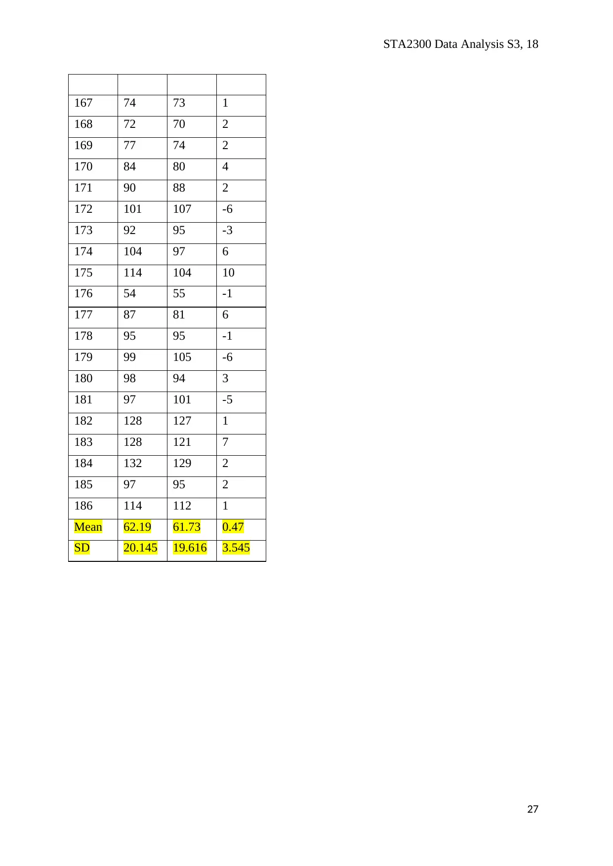
STA2300 Data Analysis S3, 18
167 74 73 1
168 72 70 2
169 77 74 2
170 84 80 4
171 90 88 2
172 101 107 -6
173 92 95 -3
174 104 97 6
175 114 104 10
176 54 55 -1
177 87 81 6
178 95 95 -1
179 99 105 -6
180 98 94 3
181 97 101 -5
182 128 127 1
183 128 121 7
184 132 129 2
185 97 95 2
186 114 112 1
Mean 62.19 61.73 0.47
SD 20.145 19.616 3.545
27
1 out of 27
Related Documents


Your All-in-One AI-Powered Toolkit for Academic Success.
+13062052269
info@desklib.com
Available 24*7 on WhatsApp / Email
![[object Object]](/_next/static/media/star-bottom.7253800d.svg)
Unlock your academic potential
© 2024 | Zucol Services PVT LTD | All rights reserved.