BUS 105 Computing Assignment: Statistical Data Analysis Report

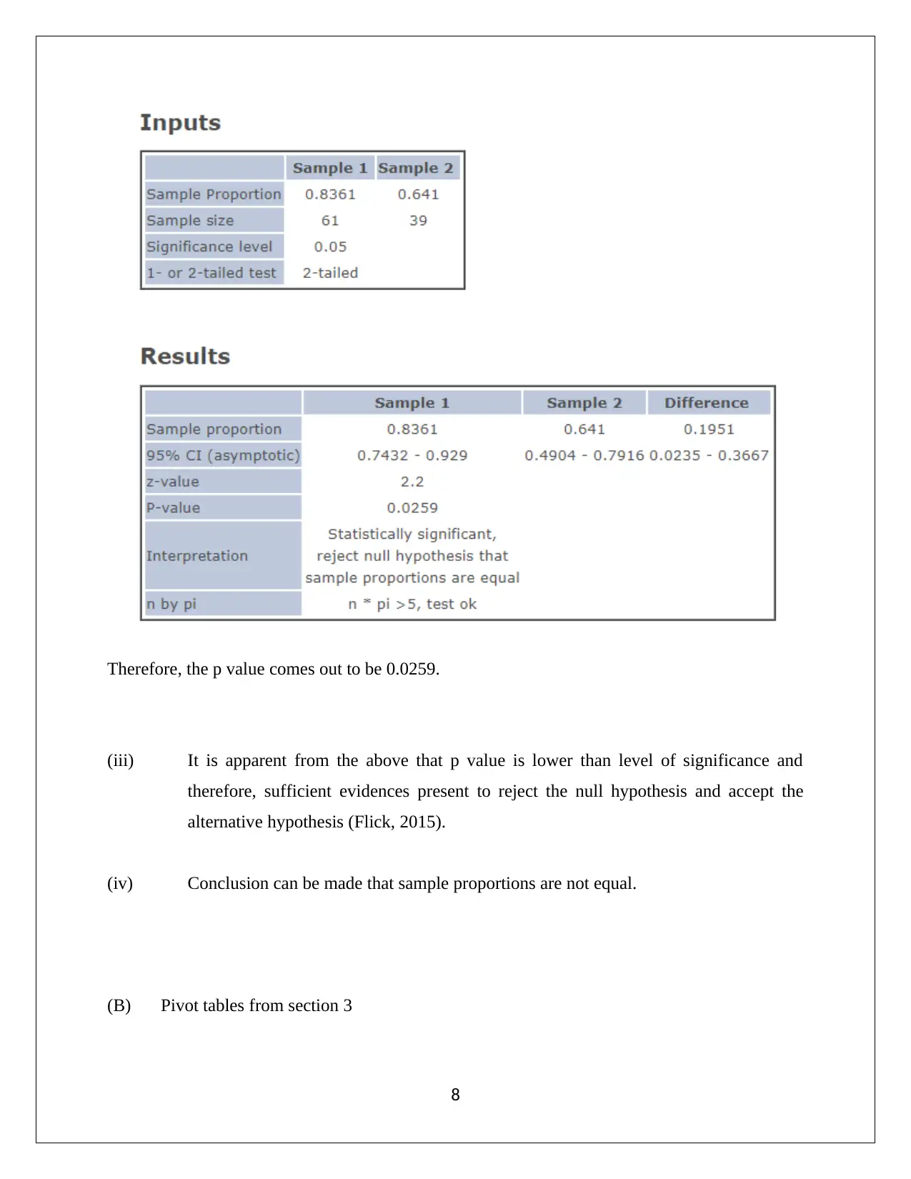
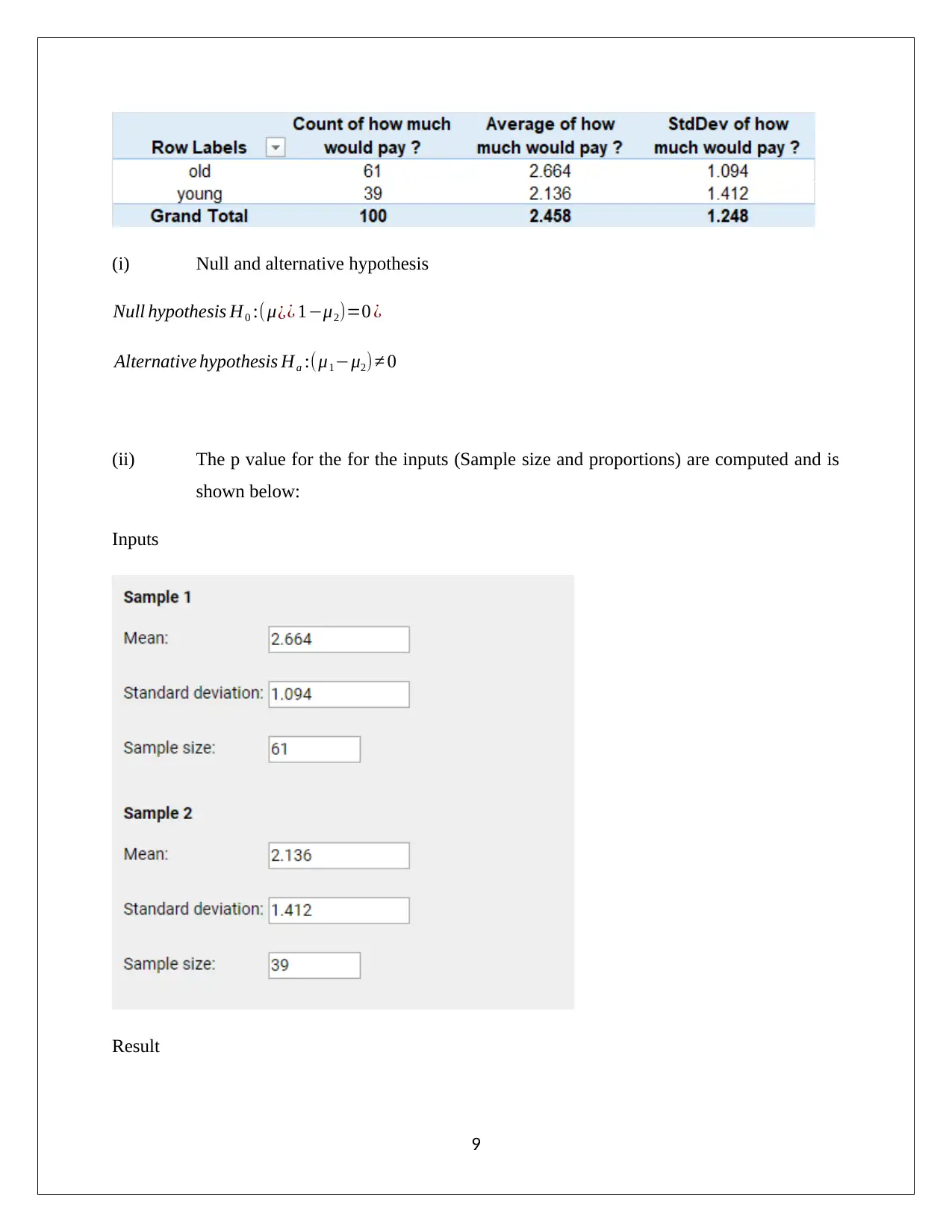
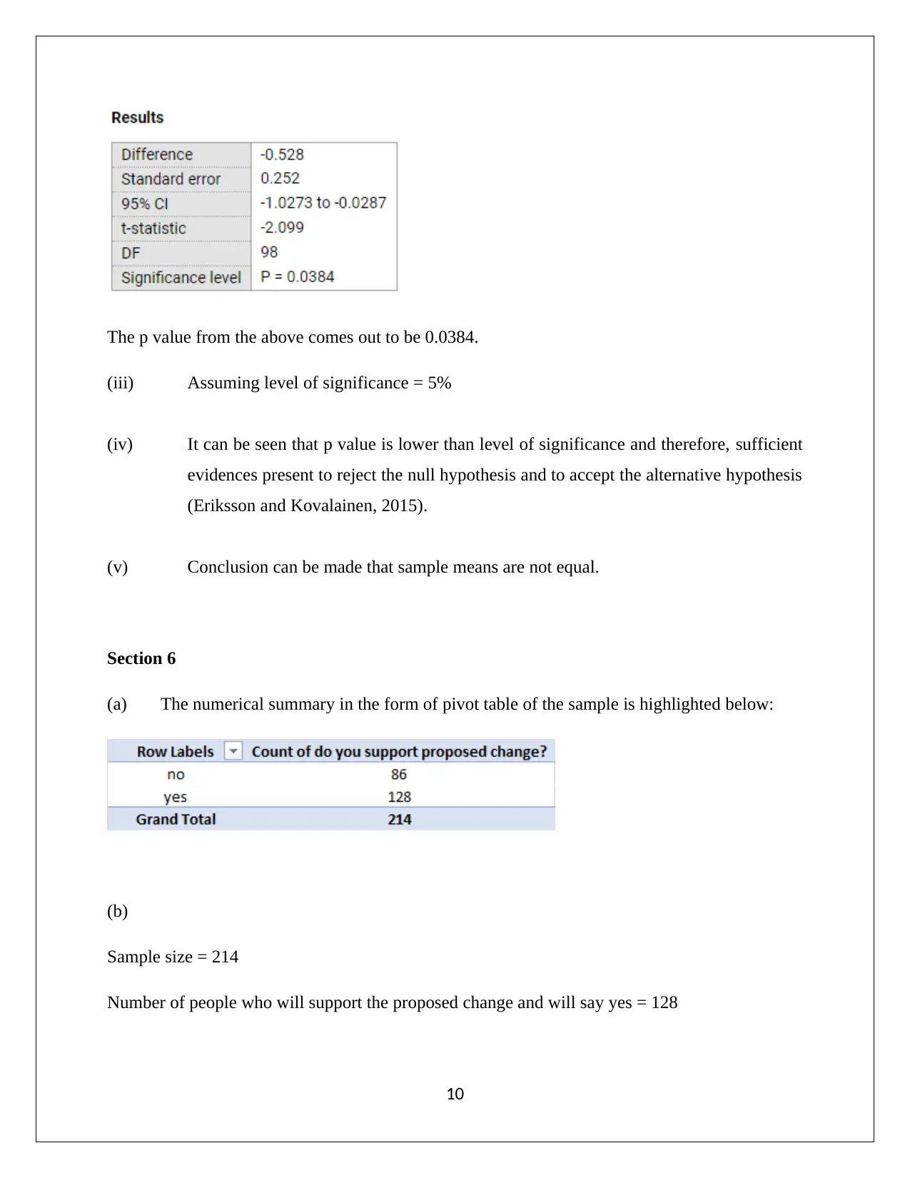
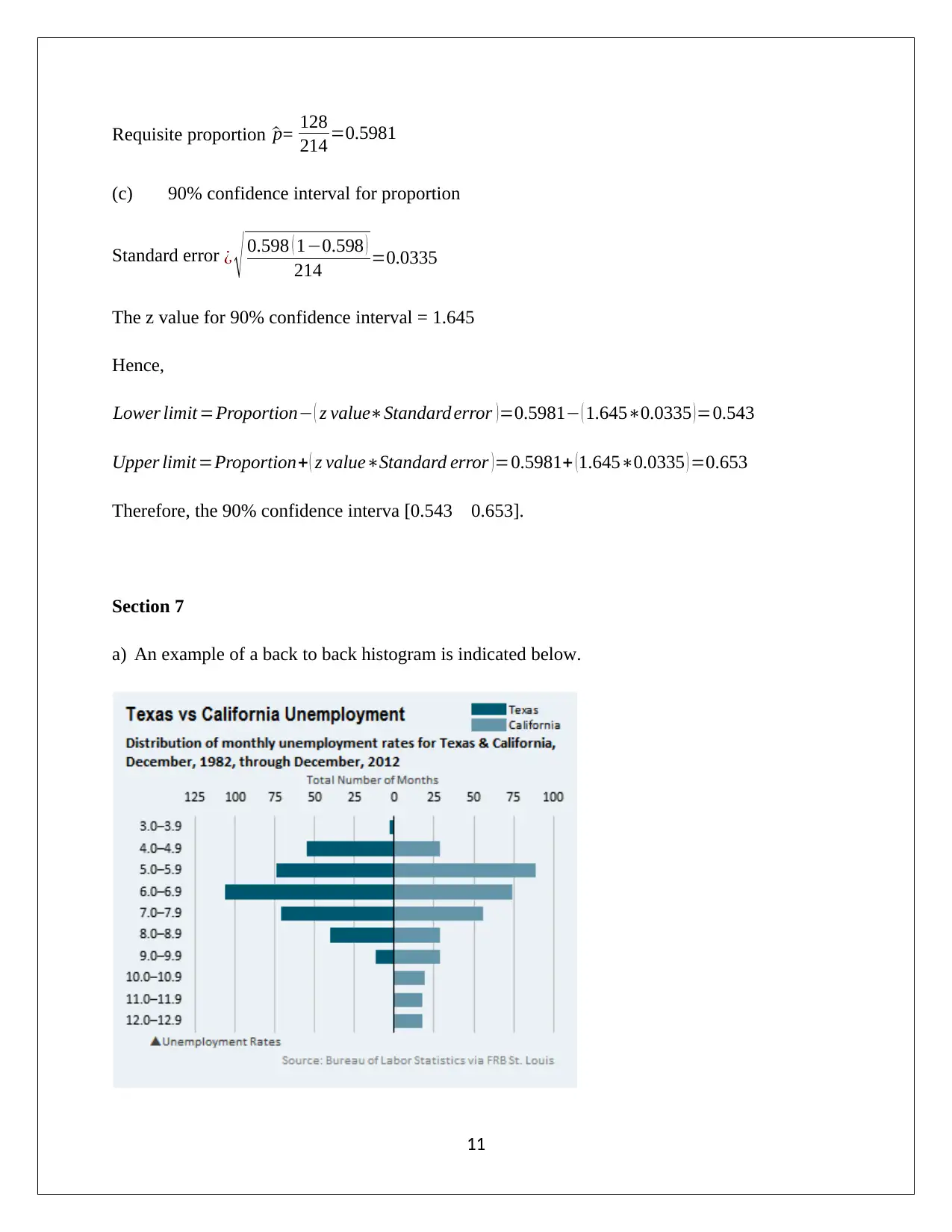
This document provides a detailed solution to a computing assignment involving statistical data analysis. The assignment covers various aspects of statistical research, including data summarization, association between variables, hypothesis testing, and confidence interval estimation. It utilizes tools like pivot tables, scatter plots, and regression analysis to interpret data and draw meaningful conclusions. The solution includes sections on comparing proportions and means, analyzing the relationship between bets and profits in a casino, and interpreting back-to-back histograms for unemployment rates. The assignment also explores hypothesis testing using p-values and discusses the implications of sampling distributions. Desklib offers a wide range of similar documents and past papers to aid students in their studies.

COMPUTING ASSIGNMENT
Waleed Usman
Student Number: 11700685
Allocated Sample: 449

Section 1
The process of statistical research is driven from dataset which consists of variables. Variables
are dynamic elements which tend to change the value. These dataset contain data captured
through requisite symbols and also highlight the values assumed. In order to ascertain the
underlying the underlying relationship and association, it is imperative to explore the variables
provided. These relationships and other summary of variables can also be found using computers
as a suitable aid mechanism (Flick, 2015).
The following data can be used as an example to illustrate the same.
The summary statistics for the above data can be found with the aid of Data Analysis option that
excel presents.
1

Also, it is possible to explore the association between the given variables through the use of
scatter diagrams as indicated below.
It is apparent that a weak positive association does tend to exist between the income and
deduction. This is apparent from the R2 and dispersion of the scatter plot points from the best fir
line. The model does not indicate a good fit (Hillier , 2016).
The use of computers is highly recommended when the amount of data to be processed is quite
high. Various software are available that can potentially summarise the data and also run various
2

inferential techniques so as to derive meaningful conclusions about the population (Hair et. al.,
2015).
Section 2
(a) The pivot tables in order to represent the relationship between age and liking for the
product is highlighted below:
Sample size of old people who would say yes for the product n1=51
Proportion of old people who would say yes for the product ^p1 =0.8361
Similarly,
Sample size of young people who would say yes for the productn2 = 25
Proportion of young people who would say yes for the product ^p2=0.6410
(b) It is apparent from the above results that there is a greater acceptability of the product
amongst consumers who are old. The acceptability of the product amongst consumers
who are young is considerably less but still substantial.
(c) The difference between the sample proportions for liking is calculated below:
3

^p1=0.8361
^p2=0.6410
Now,
Difference between the sample proportions ¿ ^p1− ^p2
^p1− ^p2=0.8361−0.6410=0.1950
Section 3
(a) The summary statistics for the sample is highlighted below:
For Old people
Sample size n1=61
Sample average x1=2.664
Sample standard deviation s1=1.094
For young people
Sample size n2 =39
Sample average x2=2.138
Sample standard deviation s2=1.412
4

(b) The average money that the old customers would pay would be higher than the
corresponding amount that young customers would pay. Also, the deviation trends seem
to be lesser for old customers as compared to young customers.
(c) Difference between the sample means x1−x2
μ1−μ2=x1 −x2=2.664−2.136
μ1−μ2=0.5280
Section 4
Data sample
(a) Scatter Plot
5

(b) There is a strong positive association between number of bets and profit and it seems that
higher number of bets does tend to lead to higher profits being earned. The coefficient of
determination is quite high indicating significant relationship between the given variables
(Eriksson and Kovalainen, 2015).
(c) Profit of casino =?
Number of bets x = 1000
Regression equation from the scatter plot
y=0.9436 x −17.625
y= ( 0.9436∗1000 )−17.625
y=925.975
Therefore, the profit of casino would be 925.975 units.
Section 5
6

(A) Pivot tables from section 2
(i) Null and alternative hypothesis
Null hypothesis H0 :( ^P¿¿ 1− ^P2)=0¿
Alternative hypothesis Ha :( ^P1 − ^P2) ≠ 0
(ii) The p value for the for the inputs (Sample size and proportions) are computed and is
shown below:
7

Therefore, the p value comes out to be 0.0259.
(iii) It is apparent from the above that p value is lower than level of significance and
therefore, sufficient evidences present to reject the null hypothesis and accept the
alternative hypothesis (Flick, 2015).
(iv) Conclusion can be made that sample proportions are not equal.
(B) Pivot tables from section 3
8

(i) Null and alternative hypothesis
Null hypothesis H0 :( μ¿¿ 1−μ2)=0 ¿
Alternative hypothesis Ha :(μ1−μ2)≠ 0
(ii) The p value for the for the inputs (Sample size and proportions) are computed and is
shown below:
Inputs
Result
9

The p value from the above comes out to be 0.0384.
(iii) Assuming level of significance = 5%
(iv) It can be seen that p value is lower than level of significance and therefore, sufficient
evidences present to reject the null hypothesis and to accept the alternative hypothesis
(Eriksson and Kovalainen, 2015).
(v) Conclusion can be made that sample means are not equal.
Section 6
(a) The numerical summary in the form of pivot table of the sample is highlighted below:
(b)
Sample size = 214
Number of people who will support the proposed change and will say yes = 128
10

Requisite proportion ^p= 128
214 =0.5981
(c) 90% confidence interval for proportion
Standard error ¿ √ 0.598 ( 1−0.598 )
214 =0.0335
The z value for 90% confidence interval = 1.645
Hence,
Lower limit =Proportion− ( z value∗Standard error )=0.5981− ( 1.645∗0.0335 )=0.543
Upper limit =Proportion+ ( z value∗Standard error )=0.5981+ (1.645∗0.0335 ) =0.653
Therefore, the 90% confidence interva [0.543 0.653].
Section 7
a) An example of a back to back histogram is indicated below.
11