Cochran (1963) Sample Size Formula History

Running head: STATISTICS 1
1
1
1
1
1
Statistics
Name
Institution
Professor
Course
Date

STATISTICS 2
Cochran (1963) sample size formula history
Cochran William developed the formula in the year 1963 for the explanation of the
sample means. According to his formula, he stated that sample means are very close to the mean
population which is highly alike. In the development of the formula, he suggested that if the null
hypothesis is not rejected there will be an expectation of the sample to be drawn close to the
population. The sample in this formula means that the normal distribution tails will be rejected
(Cochran, 2016). In this formula, in the process of testing the null hypothesis, it should be
rejected, especially when the difference between the data sample is large than what is expected.
His theory is summarized by the critical value which is at 0.7 or 7% probability for the detection
of the significant difference occurring by chance (Hoaglin, 2016).
The Cochran (1963) sample size formula is used in the calculation of the ideal sample size
provided that desired precision, estimated value, and confidence level is given. In this formula,
the confidence level is suggested to be at 93% of the attributed population sample present. This
formula is considered to be most appropriate to use especially when dealing with a large
population (Gregoire & Affleck, 2018). The sample used provided sufficient information
regarding the small population than the large one. This formula is used together with the

STATISTICS 3
correction option because the number which is provided by the Cochran formula is reducible,
especially when the population analyzed is small.
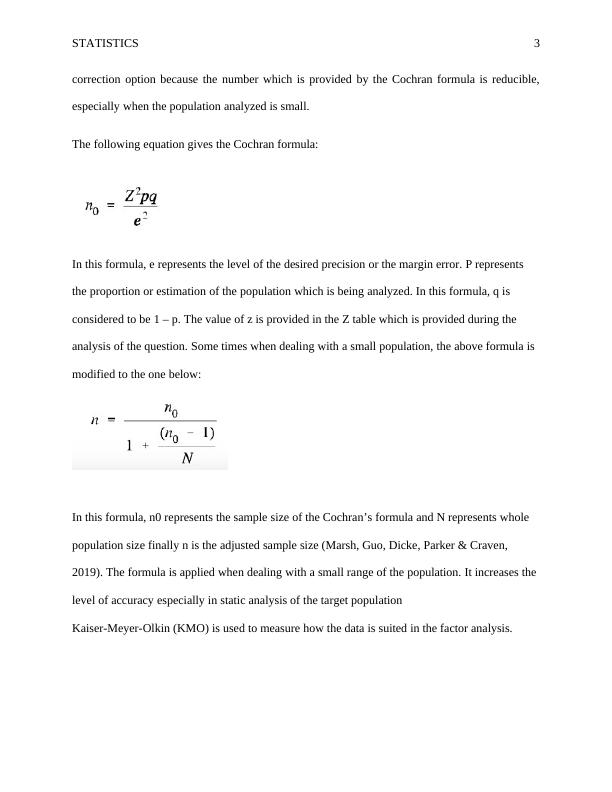
The following equation gives the Cochran formula:
In this formula, e represents the level of the desired precision or the margin error. P represents
the proportion or estimation of the population which is being analyzed. In this formula, q is
considered to be 1 – p. The value of z is provided in the Z table which is provided during the
analysis of the question. Some times when dealing with a small population, the above formula is
modified to the one below:
In this formula, n0 represents the sample size of the Cochran’s formula and N represents whole
population size finally n is the adjusted sample size (Marsh, Guo, Dicke, Parker & Craven,
2019). The formula is applied when dealing with a small range of the population. It increases the
level of accuracy especially in static analysis of the target population
Kaiser-Meyer-Olkin (KMO) is used to measure how the data is suited in the factor analysis.

STATISTICS 4
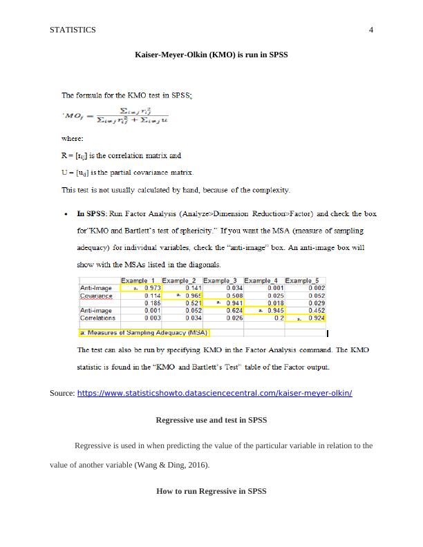
Kaiser-Meyer-Olkin (KMO) is run in SPSS
Source: https://www.statisticshowto.datasciencecentral.com/kaiser-meyer-olkin/
Regressive use and test in SPSS
Regressive is used in when predicting the value of the particular variable in relation to the
value of another variable (Wang & Ding, 2016).
How to run Regressive in SPSS