Statistics Assessment Solutions

The article provides solutions for Statistics Assessment including covariance, correlation coefficient, exponential distribution, hypothesis testing and more. The output is in json format and includes title, meta title, meta description, summary, and relevant course details.

Statistics Assessment

Answer 1:
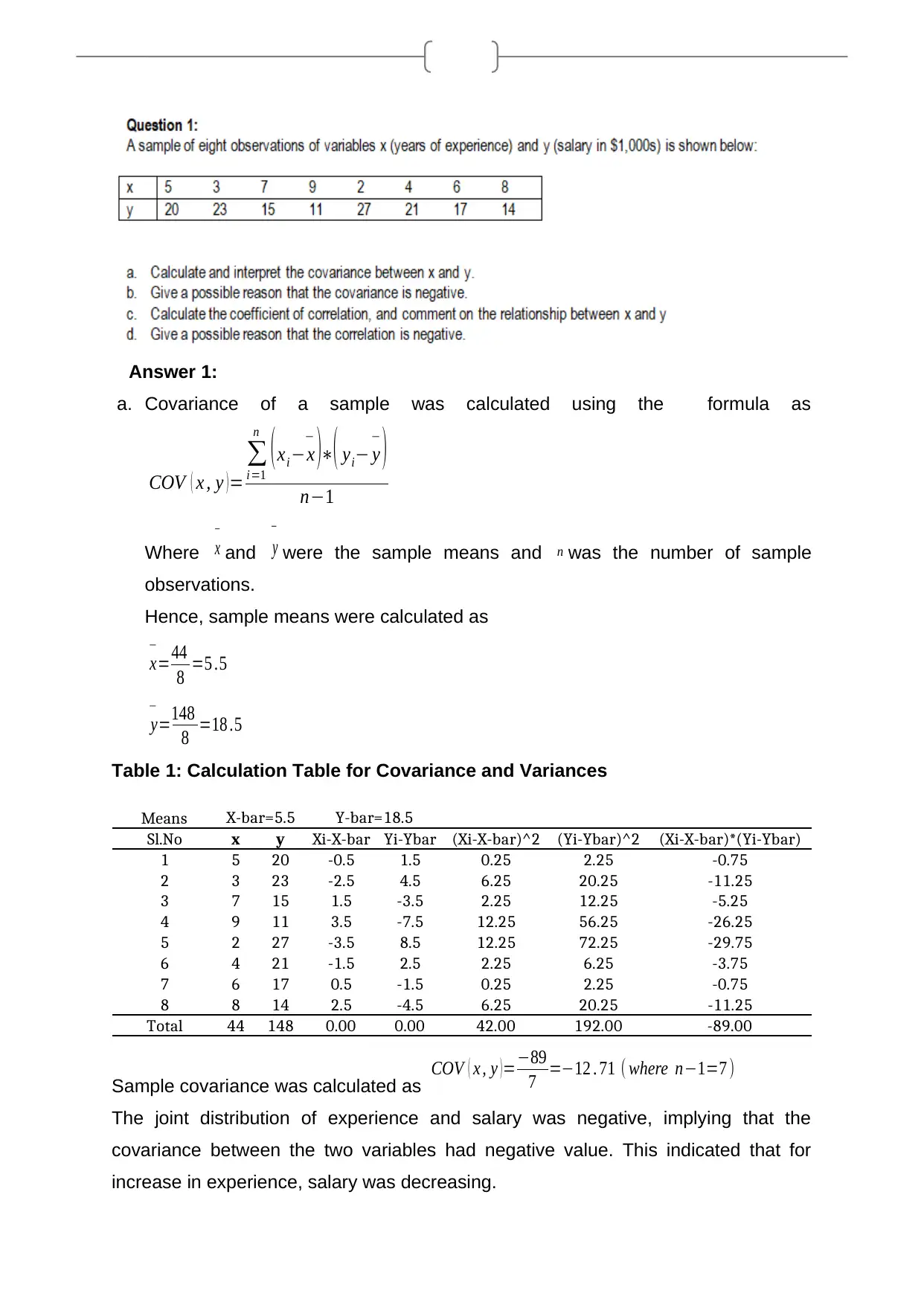
a. Covariance of a sample was calculated using the formula as
COV ( x , y ) =
∑
i=1
n
( xi−x
−
)∗( yi− y
−
)
n−1
Where x
−
and y
−
were the sample means and n was the number of sample
observations.
Hence, sample means were calculated as
x
−
=44
8 =5 .5
y
−
=148
8 =18 .5
Table 1: Calculation Table for Covariance and Variances
Means
Sl.No x y Xi-X-bar Yi-Ybar (Xi-X-bar)^2 (Yi-Ybar)^2 (Xi-X-bar)*(Yi-Ybar)
1 5 20 -0.5 1.5 0.25 2.25 -0.75
2 3 23 -2.5 4.5 6.25 20.25 -11.25
3 7 15 1.5 -3.5 2.25 12.25 -5.25
4 9 11 3.5 -7.5 12.25 56.25 -26.25
5 2 27 -3.5 8.5 12.25 72.25 -29.75
6 4 21 -1.5 2.5 2.25 6.25 -3.75
7 6 17 0.5 -1.5 0.25 2.25 -0.75
8 8 14 2.5 -4.5 6.25 20.25 -11.25
Total 44 148 0.00 0.00 42.00 192.00 -89.00
X-bar=5.5 Y-bar=18.5
Sample covariance was calculated as COV ( x , y ) =−89
7 =−12 . 71 ( where n−1=7 )
The joint distribution of experience and salary was negative, implying that the
covariance between the two variables had negative value. This indicated that for
increase in experience, salary was decreasing.

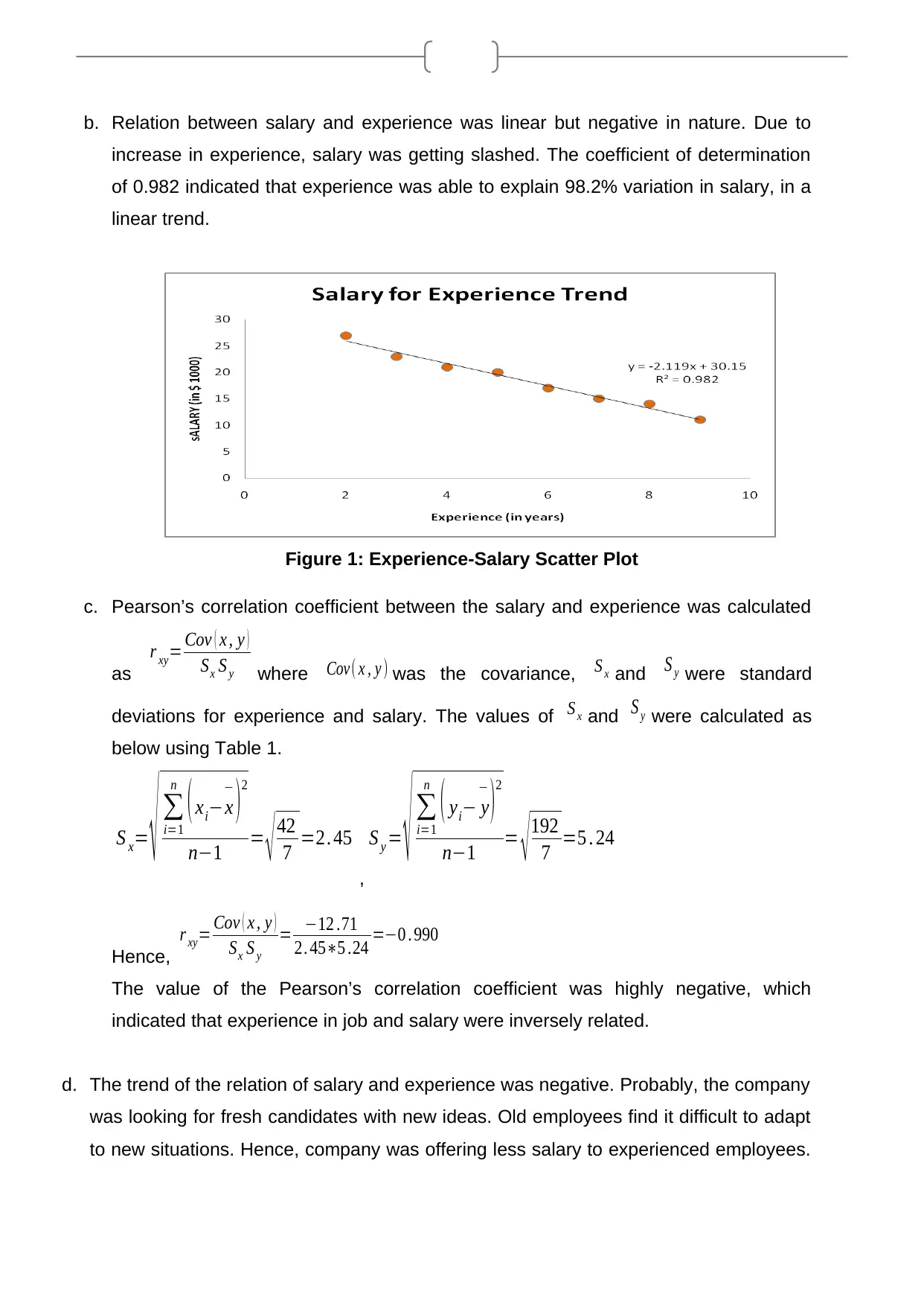
b. Relation between salary and experience was linear but negative in nature. Due to
increase in experience, salary was getting slashed. The coefficient of determination
of 0.982 indicated that experience was able to explain 98.2% variation in salary, in a
linear trend.
Figure 1: Experience-Salary Scatter Plot
c. Pearson’s correlation coefficient between the salary and experience was calculated
as
r xy= Cov ( x , y )
Sx S y where Cov( x , y ) was the covariance, S x and S y were standard
deviations for experience and salary. The values of S x and S y were calculated as
below using Table 1.
S x= √ ∑
i=1
n
( xi−x
−
)
2
n−1 = √ 42
7 =2. 45
,
S y = √ ∑
i=1
n
( yi− y
−
)
2
n−1 = √ 192
7 =5 . 24
Hence,
r xy= Cov ( x , y )
Sx S y
= −12 .71
2. 45∗5 .24 =−0 . 990
The value of the Pearson’s correlation coefficient was highly negative, which
indicated that experience in job and salary were inversely related.
d. The trend of the relation of salary and experience was negative. Probably, the company
was looking for fresh candidates with new ideas. Old employees find it difficult to adapt
to new situations. Hence, company was offering less salary to experienced employees.

Answer 2:
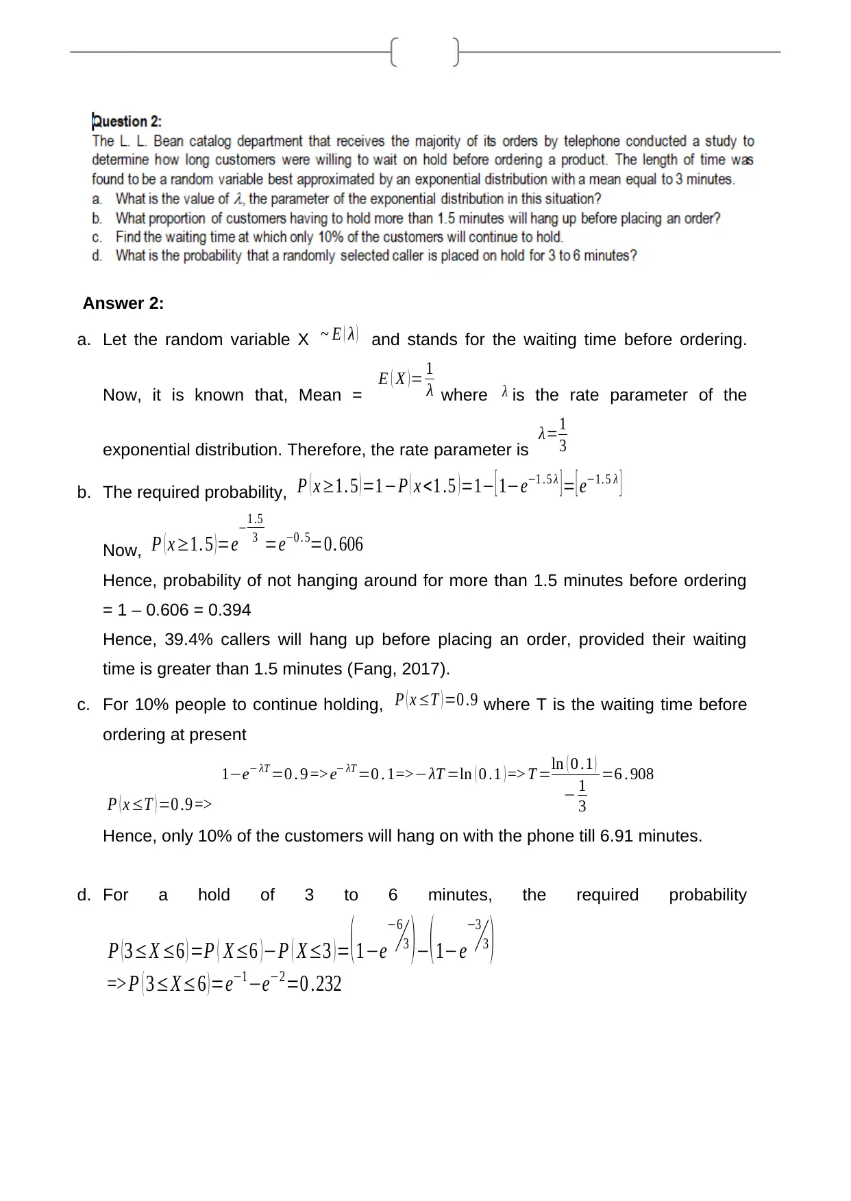
a. Let the random variable X ~ E ( λ ) and stands for the waiting time before ordering.
Now, it is known that, Mean = E ( X ) = 1
λ where λ is the rate parameter of the
exponential distribution. Therefore, the rate parameter is λ=1
3
b. The required probability, P ( x ≥1. 5 ) =1−P ( x <1 .5 ) =1− [ 1−e−1 . 5 λ ] = [ e−1. 5 λ ]
Now, P ( x ≥1. 5 ) =e−1 .5
3 =e−0 . 5=0. 606
Hence, probability of not hanging around for more than 1.5 minutes before ordering
= 1 – 0.606 = 0.394
Hence, 39.4% callers will hang up before placing an order, provided their waiting
time is greater than 1.5 minutes (Fang, 2017).
c. For 10% people to continue holding, P ( x ≤T ) =0 .9 where T is the waiting time before
ordering at present
P ( x ≤T ) =0 .9 =>
1−e− λT =0 . 9 => e− λT =0 . 1=>−λT =ln ( 0 .1 ) => T =ln ( 0 .1 )
− 1
3
=6 . 908
Hence, only 10% of the customers will hang on with the phone till 6.91 minutes.
d. For a hold of 3 to 6 minutes, the required probability
P ( 3≤X ≤6 ) =P ( X≤6 ) −P ( X≤3 ) =( 1−e
−6
3 ) −( 1−e
−3
3 )
=> P ( 3≤X≤6 ) =e−1−e−2=0 .232

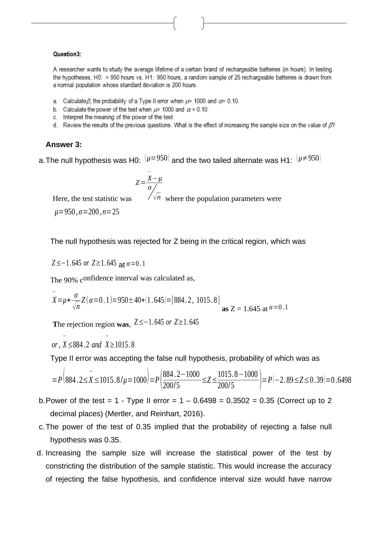
Answer 3:
a.The null hypothesis was H0: ( μ=950 ) and the two tailed alternate was H1: ( μ≠950 )
Here, the test statistic was
Z = X
−
−μ
σ
√ n where the population parameters were
μ=950 , σ=200 , n=25
The null hypothesis was rejected for Z being in the critical region, which was
Z ≤−1. 645 or Z≥1. 645 at α=0 . 1
The 90% confidence interval was calculated as,
X
−
=μ+ σ
√ n Z ( α=0 . 1)=950±40∗( 1 . 645 ) =[884 . 2 , 1015 . 8 ] as Z = 1.645 at α =0 . 1
The rejection region was, Z ≤−1. 645 or Z≥1. 645
or , X
−
≤884 . 2 and X
−
≥1015 . 8
Type II error was accepting the false null hypothesis, probability of which was as
=P ( 884 . 2≤X
−
≤1015 .8 /μ=1000 ) =P ( 884 . 2−1000
200/5 ≤Z ≤1015. 8−1000
200/ 5 )=P ( −2. 89≤Z≤0 .39 ) =0 .6498
b.Power of the test = 1 - Type II error = 1 – 0.6498 = 0.3502 = 0.35 (Correct up to 2
decimal places) (Mertler, and Reinhart, 2016).
c. The power of the test of 0.35 implied that the probability of rejecting a false null
hypothesis was 0.35.
d. Increasing the sample size will increase the statistical power of the test by
constricting the distribution of the sample statistic. This would increase the accuracy
of rejecting the false hypothesis, and confidence interval size would have narrow

down from [-2.89, 0.39].
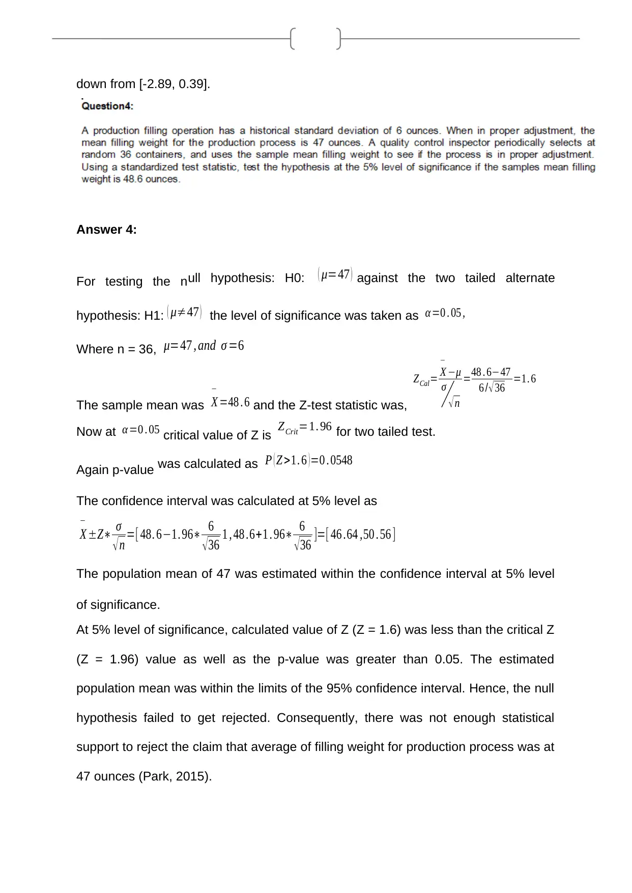
Answer 4:
For testing the null hypothesis: H0: ( μ=47 ) against the two tailed alternate
hypothesis: H1: ( μ≠47 ) the level of significance was taken as α =0 . 05 ,
Where n = 36, μ=47 , and σ =6
The sample mean was X
−
=48 . 6 and the Z-test statistic was,
ZCal= X
−
−μ
σ
√ n
=48 . 6−47
6 / √ 36 =1. 6
Now at α=0 . 05 critical value of Z is ZCrit=1. 96 for two tailed test.
Again p-value was calculated as P ( Z >1. 6 ) =0 . 0548
The confidence interval was calculated at 5% level as
X
−
±Z∗ σ
√ n =[ 48. 6−1. 96∗ 6
√ 36 1 , 48 .6+1 . 96∗ 6
√ 36 ]=[ 46 .64 ,50 . 56 ]
The population mean of 47 was estimated within the confidence interval at 5% level
of significance.
At 5% level of significance, calculated value of Z (Z = 1.6) was less than the critical Z
(Z = 1.96) value as well as the p-value was greater than 0.05. The estimated
population mean was within the limits of the 95% confidence interval. Hence, the null
hypothesis failed to get rejected. Consequently, there was not enough statistical
support to reject the claim that average of filling weight for production process was at
47 ounces (Park, 2015).

References
Fang, K.W., 2017. Symmetric Multivariate and Related Distributions: 0. Chapman
and Hall/CRC.
Mertler, C.A. and Reinhart, R.V., 2016. Advanced and multivariate statistical
methods: Practical application and interpretation. Routledge.
Park, H.M., 2015. Hypothesis testing and statistical power of a test.