Statistics Assignment: Sampling, Descriptive Statistics, Probability and Contingency Table

This assignment covers topics such as sampling, descriptive statistics, probability and contingency table. It includes a comparison of household expenses, frequency distribution of utilities, scatter plot of total expenditure and income, and contingency table of gender and education.

Running head: STATISTICS ASSIGNMENT
STATISTICS ASSIGNMENT
Name of Student
Name of University
Author Note

1STATISTICS ASSIGNMENT
Table of Contents
Task 1.........................................................................................................................................2
Task 2.........................................................................................................................................4
Task 3.........................................................................................................................................6
Task 4.........................................................................................................................................7
Reference..................................................................................................................................10

2STATISTICS ASSIGNMENT
Task 1
A. A random sample of size 250 was drawn from the given data of 2000 households on
15 variables, including expense on income excluding tax, expense on grocery, alcohol food,
fuel, cloth, phone bills, utilities, total expenditure, number of children and adults in the
household, whether the house is their own, the highest educational qualification in the
household and the gender of the household head. The data was sampled using simple random
sampling procedure.
Simple random sampling is a simple and robust process which assigns a probability
value to each individual of the population to be included in the sample. Simple random
sampling assumes that this inclusion probability is equal for all the population members. So
in a sample of size N, every person has the probability of inclusion into the sample as 1/N
and this makes the process unbiased. The process ensures that the estimate of mean is
unbiased. Moreover such probabilistic sampling methods makes it possible to objectively
measure the sampling error as well. This makes the process to be appropriate as a sampling
procedure of choice in this case (Nardi 2018).
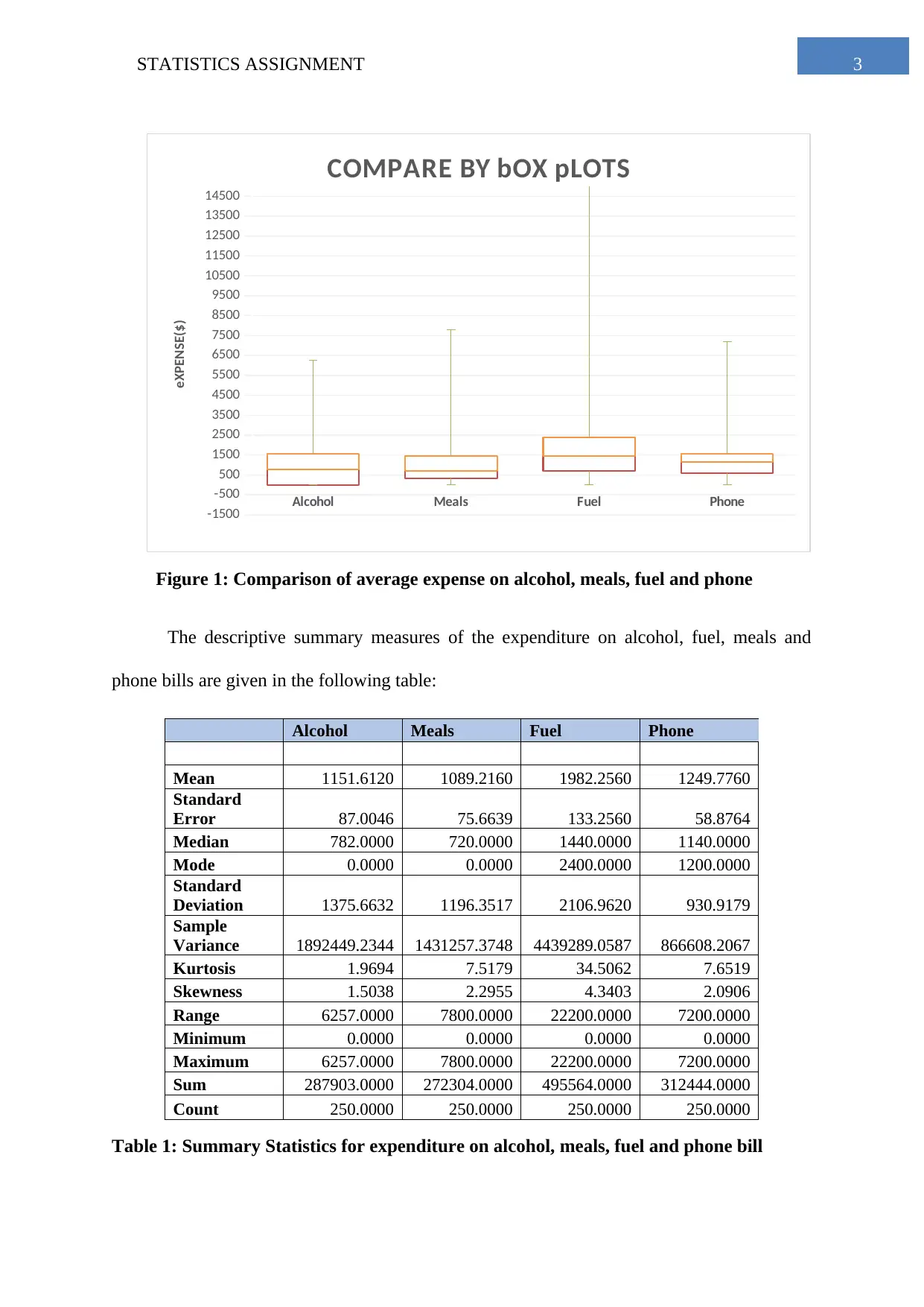
B. The following diagram shows a graphical comparison of the estimated average
expenditure of the households on fuel, alcohol, food and phone bills.

3STATISTICS ASSIGNMENT
Alcohol Meals Fuel Phone
-1500
-500
500
1500
2500
3500
4500
5500
6500
7500
8500
9500
10500
11500
12500
13500
14500
COMPARE BY bOX pLOTS
eXPENSE($)
Figure 1: Comparison of average expense on alcohol, meals, fuel and phone
The descriptive summary measures of the expenditure on alcohol, fuel, meals and
phone bills are given in the following table:
Alcohol Meals Fuel Phone
Mean 1151.6120 1089.2160 1982.2560 1249.7760
Standard
Error 87.0046 75.6639 133.2560 58.8764
Median 782.0000 720.0000 1440.0000 1140.0000
Mode 0.0000 0.0000 2400.0000 1200.0000
Standard
Deviation 1375.6632 1196.3517 2106.9620 930.9179
Sample
Variance 1892449.2344 1431257.3748 4439289.0587 866608.2067
Kurtosis 1.9694 7.5179 34.5062 7.6519
Skewness 1.5038 2.2955 4.3403 2.0906
Range 6257.0000 7800.0000 22200.0000 7200.0000
Minimum 0.0000 0.0000 0.0000 0.0000
Maximum 6257.0000 7800.0000 22200.0000 7200.0000
Sum 287903.0000 272304.0000 495564.0000 312444.0000
Count 250.0000 250.0000 250.0000 250.0000
Table 1: Summary Statistics for expenditure on alcohol, meals, fuel and phone bill

4STATISTICS ASSIGNMENT
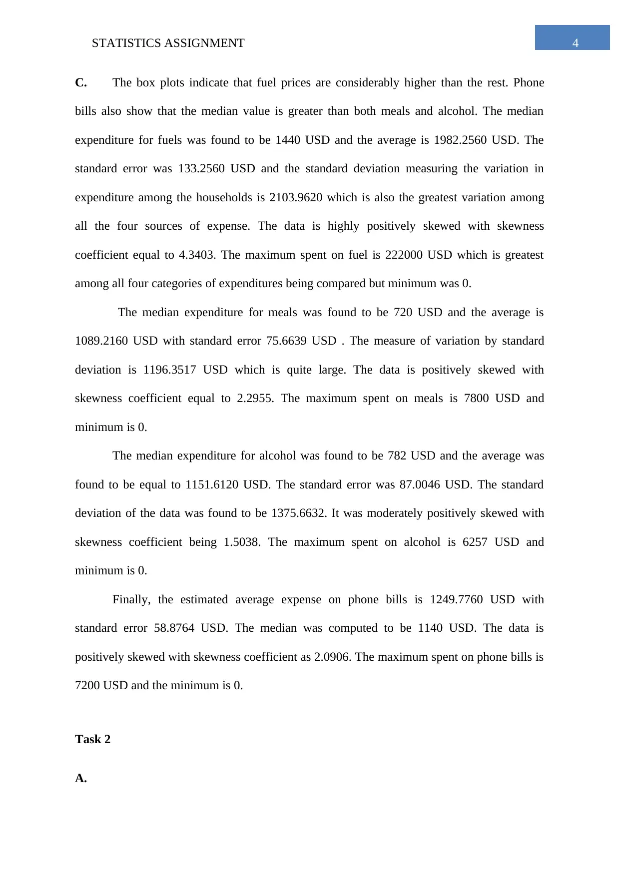
C. The box plots indicate that fuel prices are considerably higher than the rest. Phone
bills also show that the median value is greater than both meals and alcohol. The median
expenditure for fuels was found to be 1440 USD and the average is 1982.2560 USD. The
standard error was 133.2560 USD and the standard deviation measuring the variation in
expenditure among the households is 2103.9620 which is also the greatest variation among
all the four sources of expense. The data is highly positively skewed with skewness
coefficient equal to 4.3403. The maximum spent on fuel is 222000 USD which is greatest
among all four categories of expenditures being compared but minimum was 0.
The median expenditure for meals was found to be 720 USD and the average is
1089.2160 USD with standard error 75.6639 USD . The measure of variation by standard
deviation is 1196.3517 USD which is quite large. The data is positively skewed with
skewness coefficient equal to 2.2955. The maximum spent on meals is 7800 USD and
minimum is 0.
The median expenditure for alcohol was found to be 782 USD and the average was
found to be equal to 1151.6120 USD. The standard error was 87.0046 USD. The standard
deviation of the data was found to be 1375.6632. It was moderately positively skewed with
skewness coefficient being 1.5038. The maximum spent on alcohol is 6257 USD and
minimum is 0.
Finally, the estimated average expense on phone bills is 1249.7760 USD with
standard error 58.8764 USD. The median was computed to be 1140 USD. The data is
positively skewed with skewness coefficient as 2.0906. The maximum spent on phone bills is
7200 USD and the minimum is 0.
Task 2
A.

5STATISTICS ASSIGNMENT
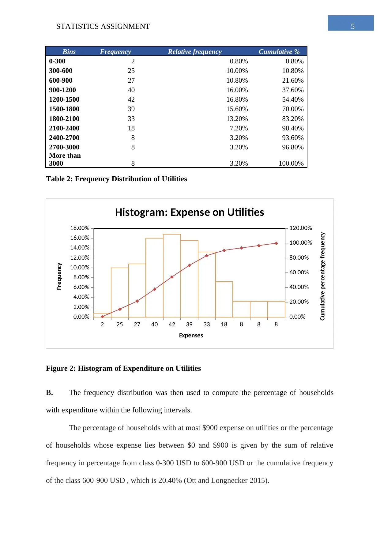
Bins Frequency Relative frequency Cumulative %
0-300 2 0.80% 0.80%
300-600 25 10.00% 10.80%
600-900 27 10.80% 21.60%
900-1200 40 16.00% 37.60%
1200-1500 42 16.80% 54.40%
1500-1800 39 15.60% 70.00%
1800-2100 33 13.20% 83.20%
2100-2400 18 7.20% 90.40%
2400-2700 8 3.20% 93.60%
2700-3000 8 3.20% 96.80%
More than
3000 8 3.20% 100.00%
Table 2: Frequency Distribution of Utilities
2 25 27 40 42 39 33 18 8 8 8
0.00%
2.00%
4.00%
6.00%
8.00%
10.00%
12.00%
14.00%
16.00%
18.00%
0.00%
20.00%
40.00%
60.00%
80.00%
100.00%
120.00%
Histogram: Expense on Utilities
Expenses
Frequency
Cumulative percentage frequency
Figure 2: Histogram of Expenditure on Utilities
B. The frequency distribution was then used to compute the percentage of households
with expenditure within the following intervals.
The percentage of households with at most $900 expense on utilities or the percentage
of households whose expense lies between $0 and $900 is given by the sum of relative
frequency in percentage from class 0-300 USD to 600-900 USD or the cumulative frequency
of the class 600-900 USD , which is 20.40% (Ott and Longnecker 2015).

6STATISTICS ASSIGNMENT
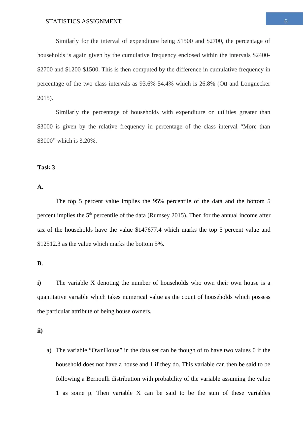
Similarly for the interval of expenditure being $1500 and $2700, the percentage of
households is again given by the cumulative frequency enclosed within the intervals $2400-
$2700 and $1200-$1500. This is then computed by the difference in cumulative frequency in
percentage of the two class intervals as 93.6%-54.4% which is 26.8% (Ott and Longnecker
2015).
Similarly the percentage of households with expenditure on utilities greater than
$3000 is given by the relative frequency in percentage of the class interval “More than
$3000” which is 3.20%.
Task 3
A.
The top 5 percent value implies the 95% percentile of the data and the bottom 5
percent implies the 5th percentile of the data (Rumsey 2015). Then for the annual income after
tax of the households have the value $147677.4 which marks the top 5 percent value and
$12512.3 as the value which marks the bottom 5%.
B.
i) The variable X denoting the number of households who own their own house is a
quantitative variable which takes numerical value as the count of households which possess
the particular attribute of being house owners.
ii)
a) The variable “OwnHouse” in the data set can be though of to have two values 0 if the
household does not have a house and 1 if they do. This variable can then be said to be
following a Bernoulli distribution with probability of the variable assuming the value
1 as some p. Then variable X can be said to be the sum of these variables

7STATISTICS ASSIGNMENT
“OwnHouse”. Then by definition of Binomial distribution, X follows Binomial (n, p).
Now for n=1, Binomial is the same as that of Bernoulli, implying that for only 1
household X has the Bernoulli distribution with parameter p (Silverman 2018).
b) When total number of households is 250, then X would have a Binomial distribution
with parameters n=250 and probability p which is same as that of the parameter of the
distribution that defines “OwnHouse”.
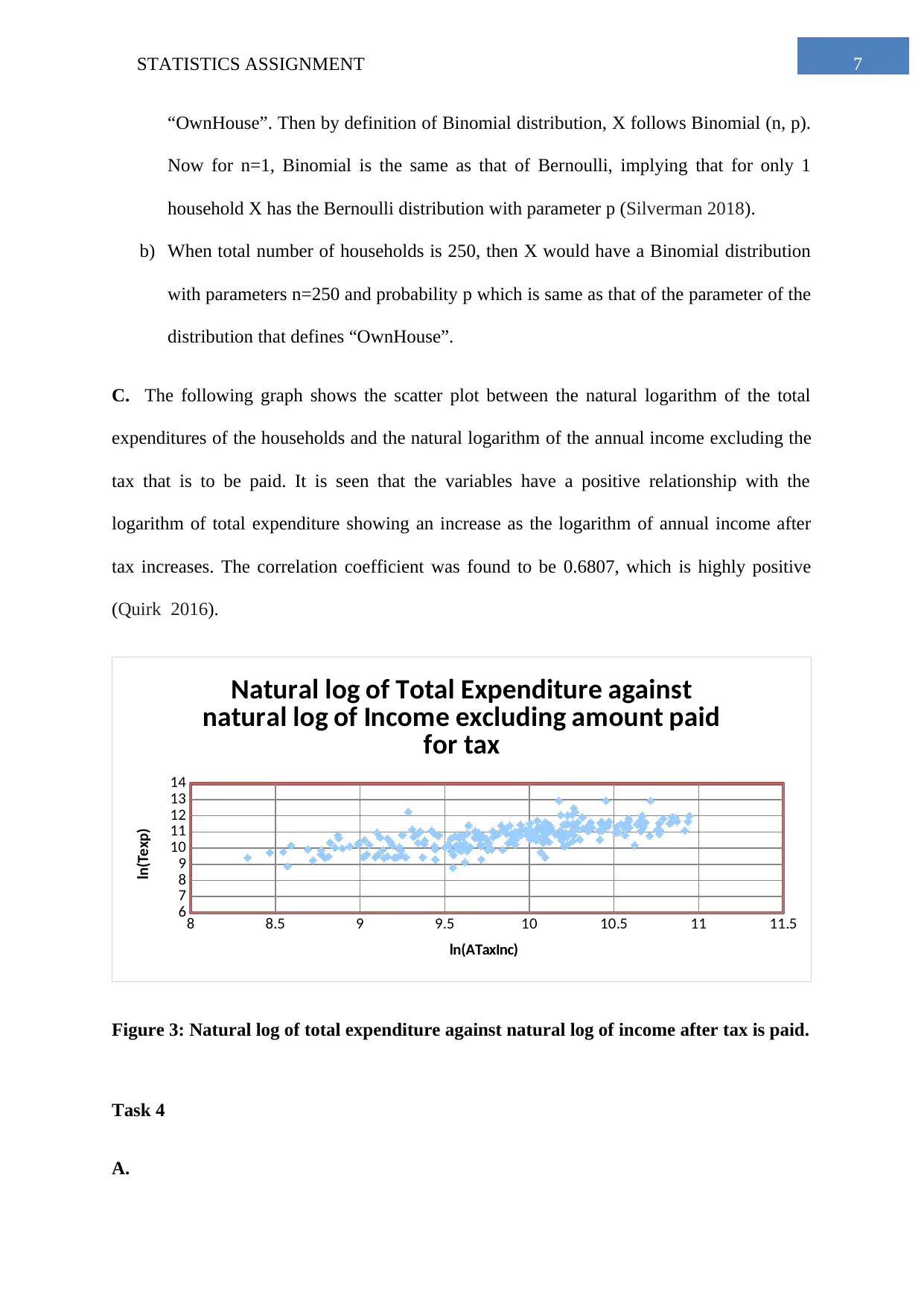
C. The following graph shows the scatter plot between the natural logarithm of the total
expenditures of the households and the natural logarithm of the annual income excluding the
tax that is to be paid. It is seen that the variables have a positive relationship with the
logarithm of total expenditure showing an increase as the logarithm of annual income after
tax increases. The correlation coefficient was found to be 0.6807, which is highly positive
(Quirk 2016).
8 8.5 9 9.5 10 10.5 11 11.5
6
7
8
9
10
11
12
13
14
Natural log of Total Expenditure against
natural log of Income excluding amount paid
for tax
ln(ATaxInc)
ln(Texp)
Figure 3: Natural log of total expenditure against natural log of income after tax is paid.
Task 4
A.

8STATISTICS ASSIGNMENT
CONTINGENCY TABLE
Gender Bachelors
Intermediat
e
Master
s
Primar
y
Secondar
y
Grand
Total
Female 0.1120 0.0800 0.0880 0.1240 0.0760 0.4800
Male 0.0320 0.1320 0.0880 0.1240 0.1440 0.5200
Grand Total 0.14 0.21 0.18 0.25 0.22 1.00
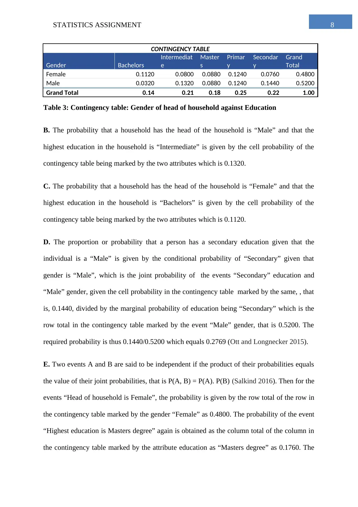
Table 3: Contingency table: Gender of head of household against Education
B. The probability that a household has the head of the household is “Male” and that the
highest education in the household is “Intermediate” is given by the cell probability of the
contingency table being marked by the two attributes which is 0.1320.
C. The probability that a household has the head of the household is “Female” and that the
highest education in the household is “Bachelors” is given by the cell probability of the
contingency table being marked by the two attributes which is 0.1120.
D. The proportion or probability that a person has a secondary education given that the
individual is a “Male” is given by the conditional probability of “Secondary” given that
gender is “Male”, which is the joint probability of the events “Secondary” education and
“Male” gender, given the cell probability in the contingency table marked by the same, , that
is, 0.1440, divided by the marginal probability of education being “Secondary” which is the
row total in the contingency table marked by the event “Male” gender, that is 0.5200. The
required probability is thus 0.1440/0.5200 which equals 0.2769 (Ott and Longnecker 2015).
E. Two events A and B are said to be independent if the product of their probabilities equals
the value of their joint probabilities, that is P(A, B) = P(A). P(B) (Salkind 2016). Then for the
events “Head of household is Female”, the probability is given by the row total of the row in
the contingency table marked by the gender “Female” as 0.4800. The probability of the event
“Highest education is Masters degree” again is obtained as the column total of the column in
the contingency table marked by the attribute education as “Masters degree” as 0.1760. The

9STATISTICS ASSIGNMENT
product of these to was found to be 0.0845. The join probability of these events is given by
the cell probability of the cell in the contingency table marked by the same which is 0.0880.
Hence the joint probability does not equal the product of the probabilities, implying that the
events are not in fact independent of each other.

10STATISTICS ASSIGNMENT
Reference
Nardi, P.M., 2018. Doing survey research: A guide to quantitative methods. Routledge.
Ott, R.L. and Longnecker, M.T., 2015. An introduction to statistical methods and data
analysis. Nelson Education.
Quirk, T.J., 2016. Excel 2016 for Engineering Statistics. Cham: Springer International
Publishing.
Rumsey, D.J., 2015. U Can: statistics for dummies. John Wiley & Sons.
Salkind, N.J., 2016. Statistics for people who (think they) hate statistics. Sage Publications.
Silverman, B.W., 2018. Density estimation for statistics and data analysis. Routledge.