Linear Regression Analysis and Optimization

This is Assignment 1 for the course ENN543 - Data Analytics and Optimisation. The assignment consists of four questions and is worth 25% of the overall subject grade. Students are required to submit their answers in a single document and upload it to TurnItIn. The assignment provides instructions on accessing the required data and submitting supplementary materials if necessary.

128 Pages10906 Words309 Views

Added on 2022-12-15

About This Document

This document discusses linear regression analysis and optimization techniques in statistics and data analytics. It covers the use of MATLAB software for linear regression analysis and provides insights into the concept of coefficients and their significance in the regression model.

Linear Regression Analysis and Optimization

Added on 2022-12-15

Related Documents

Statistics
Data Analytics and Optimisation
Solution 1:
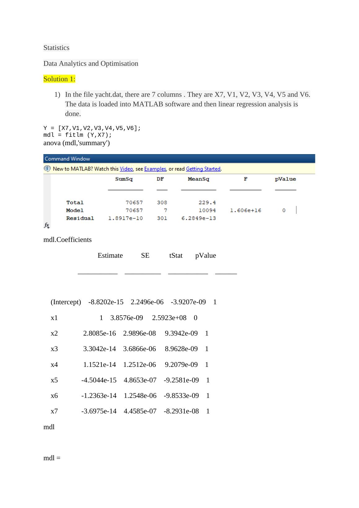
1) In the file yacht.dat, there are 7 columns . They are X7, V1, V2, V3, V4, V5 and V6.
The data is loaded into MATLAB software and then linear regression analysis is
done.
Y = [X7,V1,V2,V3,V4,V5,V6];
mdl = fitlm (Y,X7);
anova (mdl,'summary')
mdl.Coefficients
Estimate SE tStat pValue
___________ __________ ___________ ______
(Intercept) -8.8202e-15 2.2496e-06 -3.9207e-09 1
x1 1 3.8576e-09 2.5923e+08 0
x2 2.8085e-16 2.9896e-08 9.3942e-09 1
x3 3.3042e-14 3.6866e-06 8.9628e-09 1
x4 1.1521e-14 1.2512e-06 9.2079e-09 1
x5 -4.5044e-15 4.8653e-07 -9.2581e-09 1
x6 -1.2363e-14 1.2548e-06 -9.8533e-09 1
x7 -3.6975e-14 4.4585e-07 -8.2931e-08 1
mdl
mdl =

Linear Regression Analysis and Optimization_1

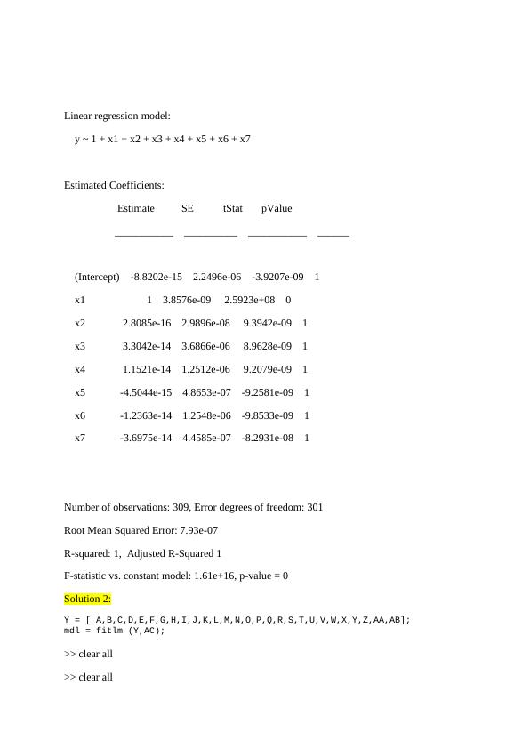
Linear regression model:
y ~ 1 + x1 + x2 + x3 + x4 + x5 + x6 + x7
Estimated Coefficients:
Estimate SE tStat pValue
___________ __________ ___________ ______
(Intercept) -8.8202e-15 2.2496e-06 -3.9207e-09 1
x1 1 3.8576e-09 2.5923e+08 0
x2 2.8085e-16 2.9896e-08 9.3942e-09 1
x3 3.3042e-14 3.6866e-06 8.9628e-09 1
x4 1.1521e-14 1.2512e-06 9.2079e-09 1
x5 -4.5044e-15 4.8653e-07 -9.2581e-09 1
x6 -1.2363e-14 1.2548e-06 -9.8533e-09 1
x7 -3.6975e-14 4.4585e-07 -8.2931e-08 1
Number of observations: 309, Error degrees of freedom: 301
Root Mean Squared Error: 7.93e-07
R-squared: 1, Adjusted R-Squared 1
F-statistic vs. constant model: 1.61e+16, p-value = 0
Solution 2:
Y = [ A,B,C,D,E,F,G,H,I,J,K,L,M,N,O,P,Q,R,S,T,U,V,W,X,Y,Z,AA,AB];
mdl = fitlm (Y,AC);
>> clear all
>> clear all

Linear Regression Analysis and Optimization_2

>> ass2a
>> mdl
mdl =
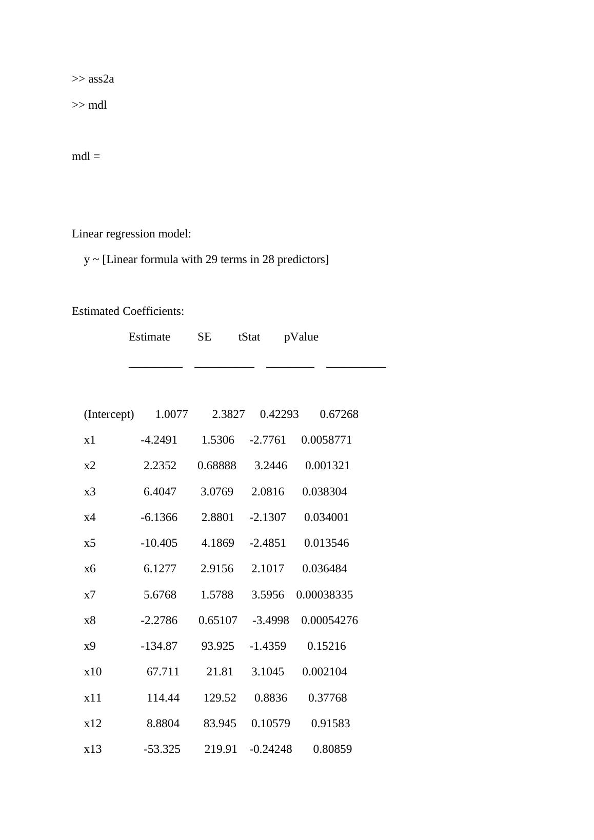
Linear regression model:
y ~ [Linear formula with 29 terms in 28 predictors]
Estimated Coefficients:
Estimate SE tStat pValue
_________ __________ ________ __________
(Intercept) 1.0077 2.3827 0.42293 0.67268
x1 -4.2491 1.5306 -2.7761 0.0058771
x2 2.2352 0.68888 3.2446 0.001321
x3 6.4047 3.0769 2.0816 0.038304
x4 -6.1366 2.8801 -2.1307 0.034001
x5 -10.405 4.1869 -2.4851 0.013546
x6 6.1277 2.9156 2.1017 0.036484
x7 5.6768 1.5788 3.5956 0.00038335
x8 -2.2786 0.65107 -3.4998 0.00054276
x9 -134.87 93.925 -1.4359 0.15216
x10 67.711 21.81 3.1045 0.002104
x11 114.44 129.52 0.8836 0.37768
x12 8.8804 83.945 0.10579 0.91583
x13 -53.325 219.91 -0.24248 0.80859

Linear Regression Analysis and Optimization_3

x14 -48.762 87.788 -0.55545 0.57904
x15 135.96 62.327 2.1814 0.029994
x16 -49.978 19.968 -2.5029 0.012897
x17 0.1957 0.070501 2.7759 0.0058814
x18 0.40697 0.06475 6.2853 1.2724e-09
x19 -0.28848 0.06858 -4.2064 3.511e-05
x20 0.058848 0.053679 1.0963 0.2739
x21 -14.353 5.1388 -2.7932 0.0055845
x22 -8.324 2.3417 -3.5546 0.00044517
x23 -2.7275 2.5477 -1.0706 0.28531
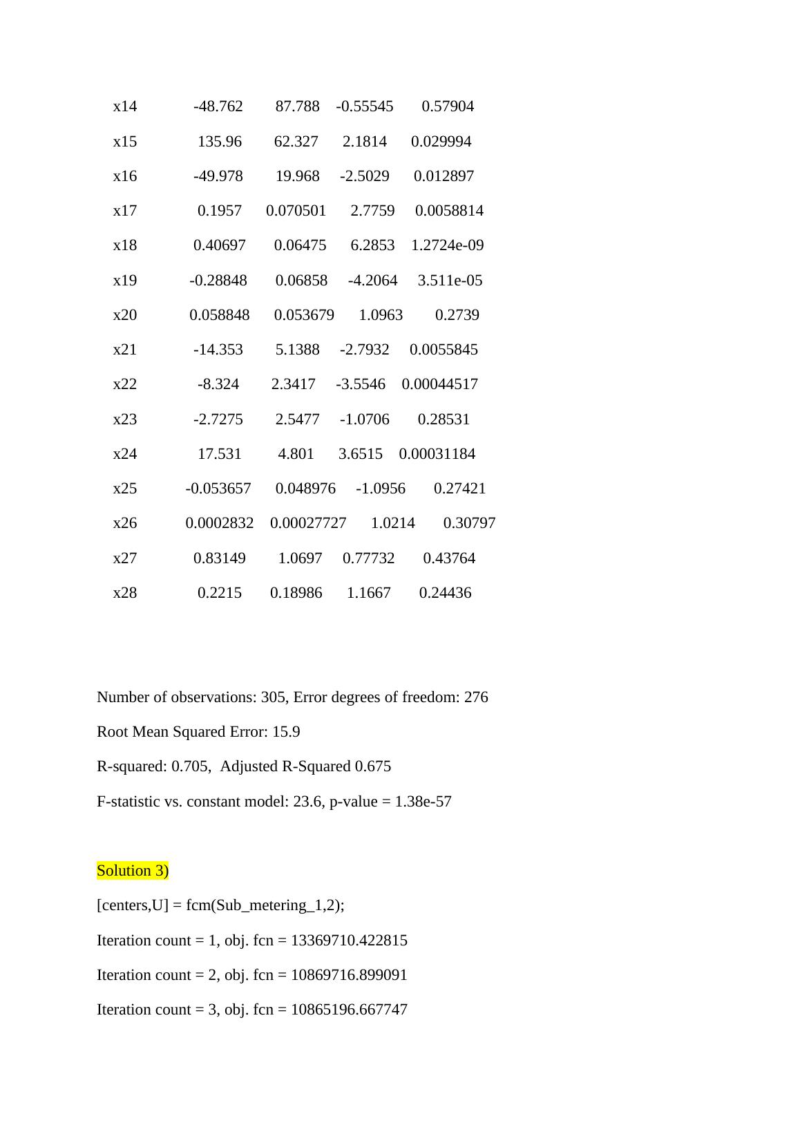
x24 17.531 4.801 3.6515 0.00031184
x25 -0.053657 0.048976 -1.0956 0.27421
x26 0.0002832 0.00027727 1.0214 0.30797
x27 0.83149 1.0697 0.77732 0.43764
x28 0.2215 0.18986 1.1667 0.24436
Number of observations: 305, Error degrees of freedom: 276
Root Mean Squared Error: 15.9
R-squared: 0.705, Adjusted R-Squared 0.675
F-statistic vs. constant model: 23.6, p-value = 1.38e-57
Solution 3)
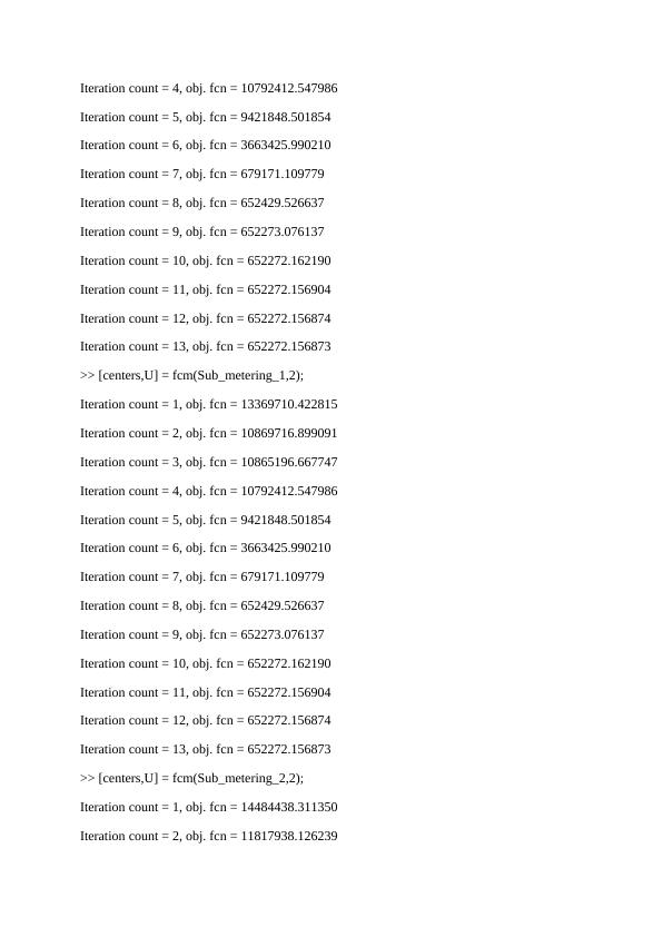
[centers,U] = fcm(Sub_metering_1,2);
Iteration count = 1, obj. fcn = 13369710.422815
Iteration count = 2, obj. fcn = 10869716.899091
Iteration count = 3, obj. fcn = 10865196.667747

Linear Regression Analysis and Optimization_4

Iteration count = 4, obj. fcn = 10792412.547986
Iteration count = 5, obj. fcn = 9421848.501854
Iteration count = 6, obj. fcn = 3663425.990210
Iteration count = 7, obj. fcn = 679171.109779
Iteration count = 8, obj. fcn = 652429.526637
Iteration count = 9, obj. fcn = 652273.076137
Iteration count = 10, obj. fcn = 652272.162190
Iteration count = 11, obj. fcn = 652272.156904
Iteration count = 12, obj. fcn = 652272.156874
Iteration count = 13, obj. fcn = 652272.156873
>> [centers,U] = fcm(Sub_metering_1,2);
Iteration count = 1, obj. fcn = 13369710.422815
Iteration count = 2, obj. fcn = 10869716.899091
Iteration count = 3, obj. fcn = 10865196.667747
Iteration count = 4, obj. fcn = 10792412.547986
Iteration count = 5, obj. fcn = 9421848.501854
Iteration count = 6, obj. fcn = 3663425.990210
Iteration count = 7, obj. fcn = 679171.109779
Iteration count = 8, obj. fcn = 652429.526637
Iteration count = 9, obj. fcn = 652273.076137
Iteration count = 10, obj. fcn = 652272.162190
Iteration count = 11, obj. fcn = 652272.156904
Iteration count = 12, obj. fcn = 652272.156874
Iteration count = 13, obj. fcn = 652272.156873
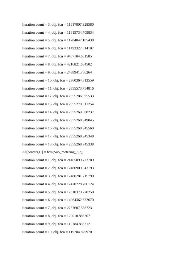
>> [centers,U] = fcm(Sub_metering_2,2);
Iteration count = 1, obj. fcn = 14484438.311350
Iteration count = 2, obj. fcn = 11817938.126239

Linear Regression Analysis and Optimization_5

Iteration count = 3, obj. fcn = 11817807.928580
Iteration count = 4, obj. fcn = 11815734.709834
Iteration count = 5, obj. fcn = 11784847.105438
Iteration count = 6, obj. fcn = 11493327.814107
Iteration count = 7, obj. fcn = 9457104.651585
Iteration count = 8, obj. fcn = 4216821.684502
Iteration count = 9, obj. fcn = 2438941.786264
Iteration count = 10, obj. fcn = 2360364.313559
Iteration count = 11, obj. fcn = 2355573.754816
Iteration count = 12, obj. fcn = 2355286.995533
Iteration count = 13, obj. fcn = 2355270.011254
Iteration count = 14, obj. fcn = 2355269.008237
Iteration count = 15, obj. fcn = 2355268.949045
Iteration count = 16, obj. fcn = 2355268.945560
Iteration count = 17, obj. fcn = 2355268.945348
Iteration count = 18, obj. fcn = 2355268.945338
>>[centers,U] = fcm(Sub_metering_3,2);
Iteration count = 1, obj. fcn = 21465899.723789
Iteration count = 2, obj. fcn = 17480909.843193
Iteration count = 3, obj. fcn = 17480281.215790
Iteration count = 4, obj. fcn = 17470228.286124
Iteration count = 5, obj. fcn = 17310379.270250
Iteration count = 6, obj. fcn = 14964362.632670
Iteration count = 7, obj. fcn = 2767607.558723
Iteration count = 8, obj. fcn = 120010.885307
Iteration count = 9, obj. fcn = 119784.838312
Iteration count = 10, obj. fcn = 119784.829970

Linear Regression Analysis and Optimization_6

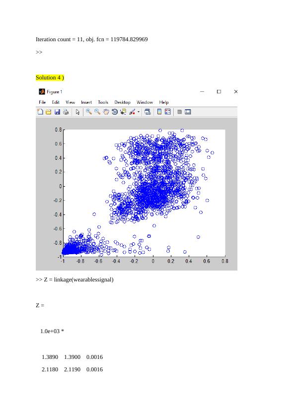
Iteration count = 11, obj. fcn = 119784.829969
>>
Solution 4 )
>> Z = linkage(wearablessignal)
Z =
1.0e+03 *
1.3890 1.3900 0.0016
2.1180 2.1190 0.0016

Linear Regression Analysis and Optimization_7

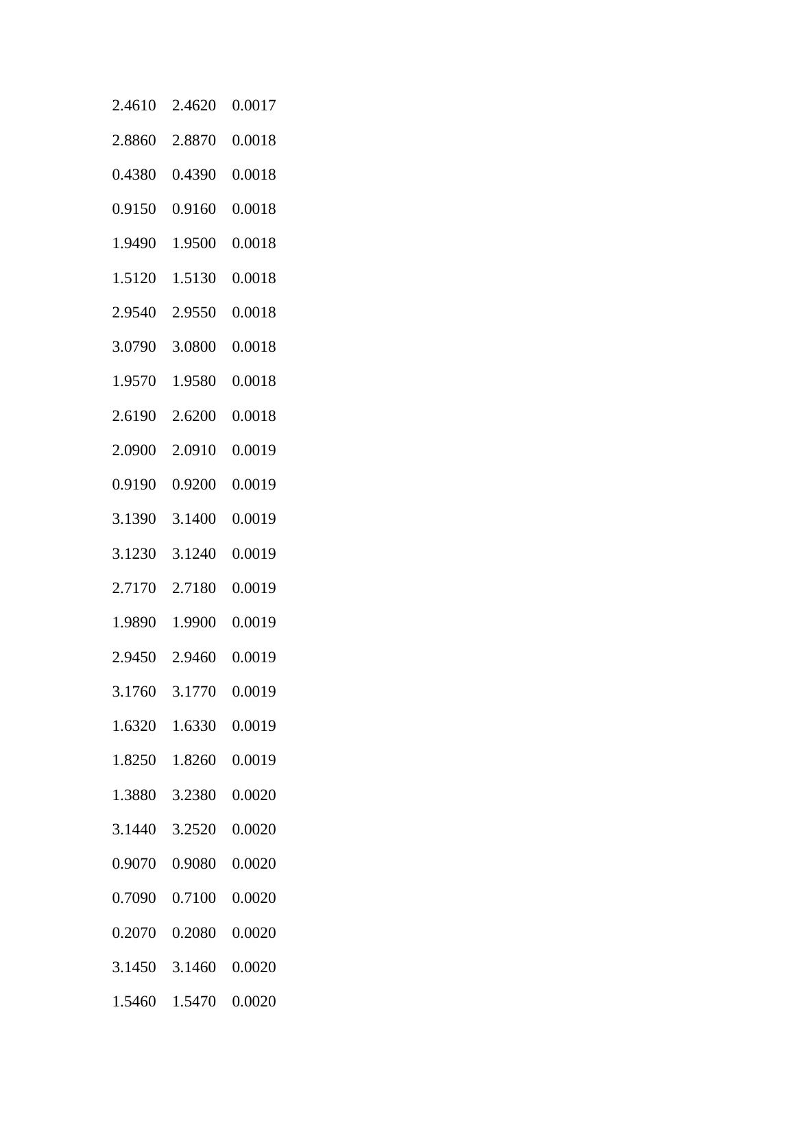
2.4610 2.4620 0.0017
2.8860 2.8870 0.0018
0.4380 0.4390 0.0018
0.9150 0.9160 0.0018
1.9490 1.9500 0.0018
1.5120 1.5130 0.0018
2.9540 2.9550 0.0018
3.0790 3.0800 0.0018
1.9570 1.9580 0.0018
2.6190 2.6200 0.0018
2.0900 2.0910 0.0019
0.9190 0.9200 0.0019
3.1390 3.1400 0.0019
3.1230 3.1240 0.0019
2.7170 2.7180 0.0019
1.9890 1.9900 0.0019
2.9450 2.9460 0.0019
3.1760 3.1770 0.0019
1.6320 1.6330 0.0019
1.8250 1.8260 0.0019
1.3880 3.2380 0.0020
3.1440 3.2520 0.0020
0.9070 0.9080 0.0020
0.7090 0.7100 0.0020
0.2070 0.2080 0.0020
3.1450 3.1460 0.0020
1.5460 1.5470 0.0020

Linear Regression Analysis and Optimization_8

End of preview

Want to access all the pages? Upload your documents or become a member.

Linear Regression Model for Resistance per Unit Weight of Displacement

|106

|14401

|57

Assignment on econometrics PDF

|28

|4390

|481

Cox Proportional Hazards Model for Survival Analysis

|876

|350

Design Optimisation for Manufacturing

|10

|1615

|51

Business Analytics

|17

|1844

|77

Regression Analysis Assignment Pdf - Statistics 2022

|673

|115

Linear Regression Analysis and Optimization

About This Document

Linear Regression Analysis and Optimization

End of preview

Linear Regression Model for Resistance per Unit Weight of Displacementlg...

Assignment on econometrics PDFlg...

Cox Proportional Hazards Model for Survival Analysislg...

Design Optimisation for Manufacturinglg...

Business Analyticslg...

Regression Analysis Assignment Pdf - Statistics 2022lg...

Linear Regression Model for Resistance per Unit Weight of Displacement

Assignment on econometrics PDF

Cox Proportional Hazards Model for Survival Analysis

Design Optimisation for Manufacturing

Business Analytics

Regression Analysis Assignment Pdf - Statistics 2022