Regression Analysis for Price and Sales

This document provides a detailed analysis of regression models for two different scenarios - one involving the relationship between price and sales, and the other involving the effects of various variables on house prices. It includes regression outputs, hypothesis testing, interpretation of slopes, confidence intervals, and forecasting demand.

STATISTICS
[Document subtitle]
[DATE]

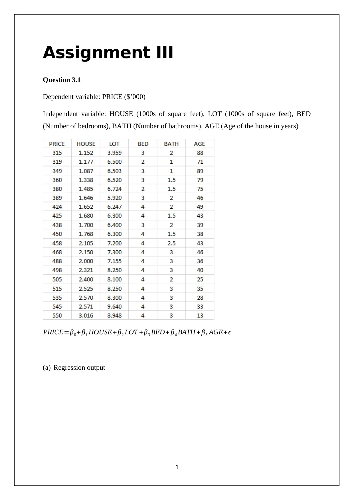
Assignment III
Question 3.1
Dependent variable: PRICE ($’000)
Independent variable: HOUSE (1000s of square feet), LOT (1000s of square feet), BED
(Number of bedrooms), BATH (Number of bathrooms), AGE (Age of the house in years)
PRICE=β0 + β1 HOUSE +β2 LOT +β3 BED+ β4 BATH + β5 AGE+ ϵ
(a) Regression output
1

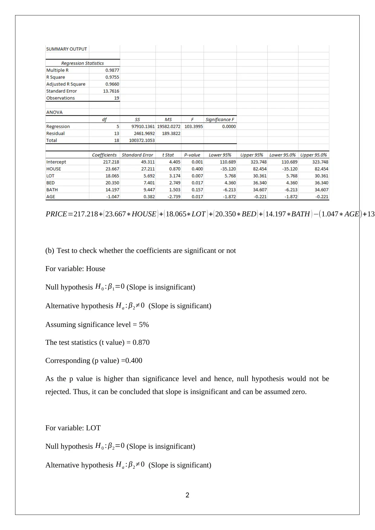
PRICE=217.218+ ( 23.667∗HOUSE ) + ( 18.065∗LOT ) + ( 20.350∗BED ) + ( 14.197∗BATH ) −(1.047∗AGE)+13
(b) Test to check whether the coefficients are significant or not
For variable: House
Null hypothesis H0 : β1=0 (Slope is insignificant)
Alternative hypothesis Ha : β2 ≠ 0 (Slope is significant)
Assuming significance level = 5%
The test statistics (t value) = 0.870
Corresponding (p value) =0.400
As the p value is higher than significance level and hence, null hypothesis would not be
rejected. Thus, it can be concluded that slope is insignificant and can be assumed zero.
For variable: LOT
Null hypothesis H0 : β2=0 (Slope is insignificant)
Alternative hypothesis Ha : β2 ≠ 0 (Slope is significant)
2

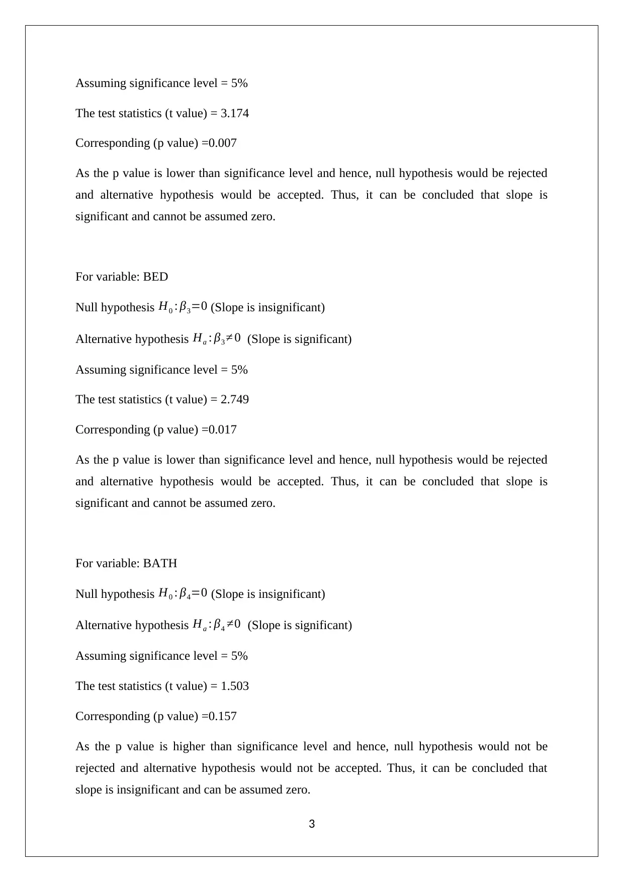
Assuming significance level = 5%
The test statistics (t value) = 3.174
Corresponding (p value) =0.007
As the p value is lower than significance level and hence, null hypothesis would be rejected
and alternative hypothesis would be accepted. Thus, it can be concluded that slope is
significant and cannot be assumed zero.
For variable: BED
Null hypothesis H0 : β3=0 (Slope is insignificant)
Alternative hypothesis Ha : β3 ≠ 0 (Slope is significant)
Assuming significance level = 5%
The test statistics (t value) = 2.749
Corresponding (p value) =0.017
As the p value is lower than significance level and hence, null hypothesis would be rejected
and alternative hypothesis would be accepted. Thus, it can be concluded that slope is
significant and cannot be assumed zero.
For variable: BATH
Null hypothesis H0 : β4=0 (Slope is insignificant)
Alternative hypothesis Ha : β4 ≠0 (Slope is significant)
Assuming significance level = 5%
The test statistics (t value) = 1.503
Corresponding (p value) =0.157
As the p value is higher than significance level and hence, null hypothesis would not be
rejected and alternative hypothesis would not be accepted. Thus, it can be concluded that
slope is insignificant and can be assumed zero.
3

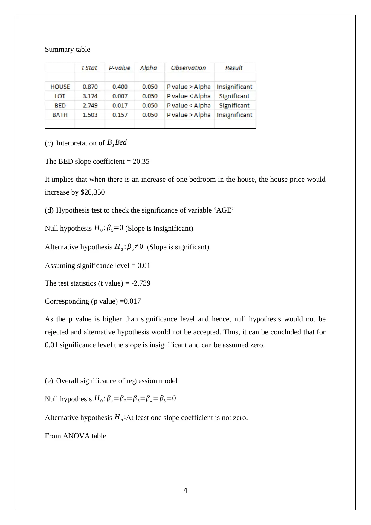
Summary table
(c) Interpretation of Β3 Bed
The BED slope coefficient = 20.35
It implies that when there is an increase of one bedroom in the house, the house price would
increase by $20,350
(d) Hypothesis test to check the significance of variable ‘AGE’
Null hypothesis H0 : β5=0 (Slope is insignificant)
Alternative hypothesis Ha : β5 ≠ 0 (Slope is significant)
Assuming significance level = 0.01
The test statistics (t value) = -2.739
Corresponding (p value) =0.017
As the p value is higher than significance level and hence, null hypothesis would not be
rejected and alternative hypothesis would not be accepted. Thus, it can be concluded that for
0.01 significance level the slope is insignificant and can be assumed zero.
(e) Overall significance of regression model
Null hypothesis H0 : β1=β2=β3=β4= β5 =0
Alternative hypothesis Ha :At least one slope coefficient is not zero.
From ANOVA table
4

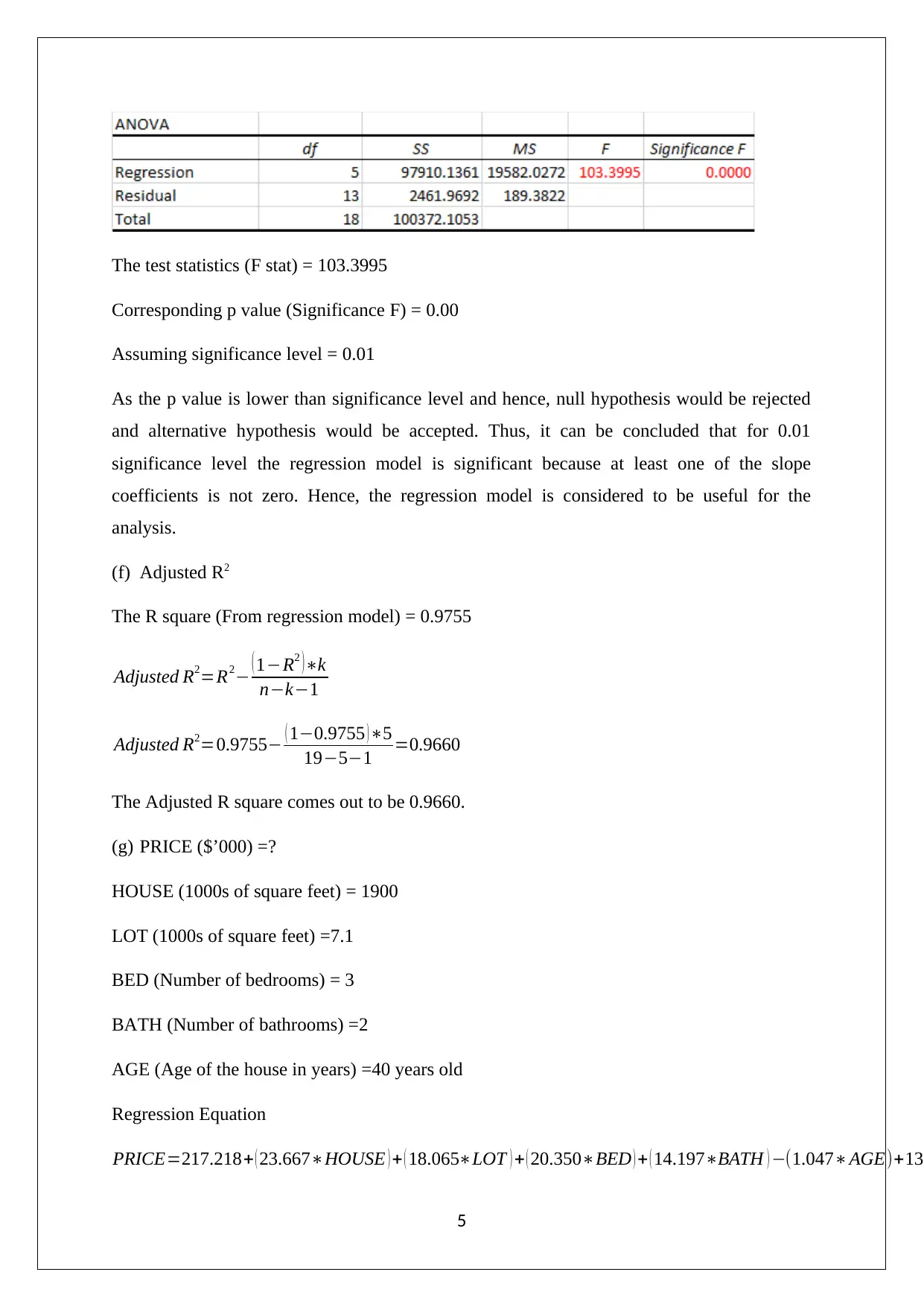
The test statistics (F stat) = 103.3995
Corresponding p value (Significance F) = 0.00
Assuming significance level = 0.01
As the p value is lower than significance level and hence, null hypothesis would be rejected
and alternative hypothesis would be accepted. Thus, it can be concluded that for 0.01
significance level the regression model is significant because at least one of the slope
coefficients is not zero. Hence, the regression model is considered to be useful for the
analysis.
(f) Adjusted R2
The R square (From regression model) = 0.9755
Adjusted R2=R2− ( 1−R2 ) ∗k
n−k−1
Adjusted R2=0.9755− ( 1−0.9755 ) ∗5
19−5−1 =0.9660
The Adjusted R square comes out to be 0.9660.
(g) PRICE ($’000) =?
HOUSE (1000s of square feet) = 1900
LOT (1000s of square feet) =7.1
BED (Number of bedrooms) = 3
BATH (Number of bathrooms) =2
AGE (Age of the house in years) =40 years old
Regression Equation
PRICE=217.218+ ( 23.667∗HOUSE ) + ( 18.065∗LOT ) + ( 20.350∗BED ) + ( 14.197∗BATH ) −(1.047∗AGE)+13
5

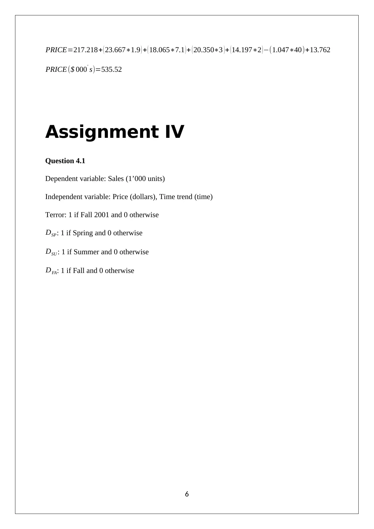
PRICE=217.218+ ( 23.667∗1.9 ) + ( 18.065∗7.1 ) + ( 20.350∗3 ) + ( 14.197∗2 ) −(1.047∗40)+13.762
PRICE ($ 000' s)=535.52
Assignment IV
Question 4.1
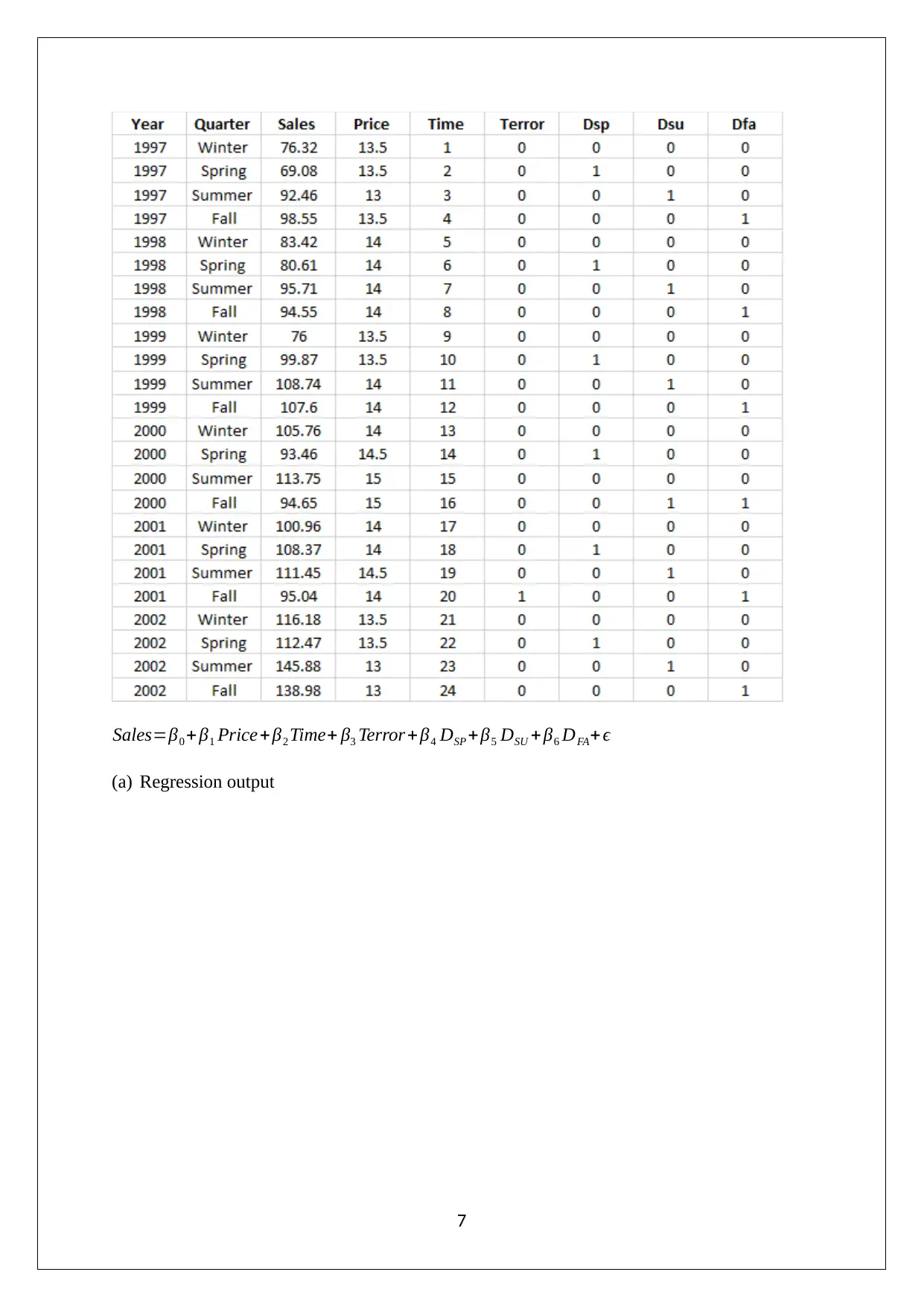
Dependent variable: Sales (1’000 units)
Independent variable: Price (dollars), Time trend (time)
Terror: 1 if Fall 2001 and 0 otherwise
DSP: 1 if Spring and 0 otherwise
DSU : 1 if Summer and 0 otherwise
DFA: 1 if Fall and 0 otherwise
6

Sales=β0 + β1 Price+β2 Time+ β3 Terror + β4 DSP + β5 DSU +β6 DFA+ ϵ
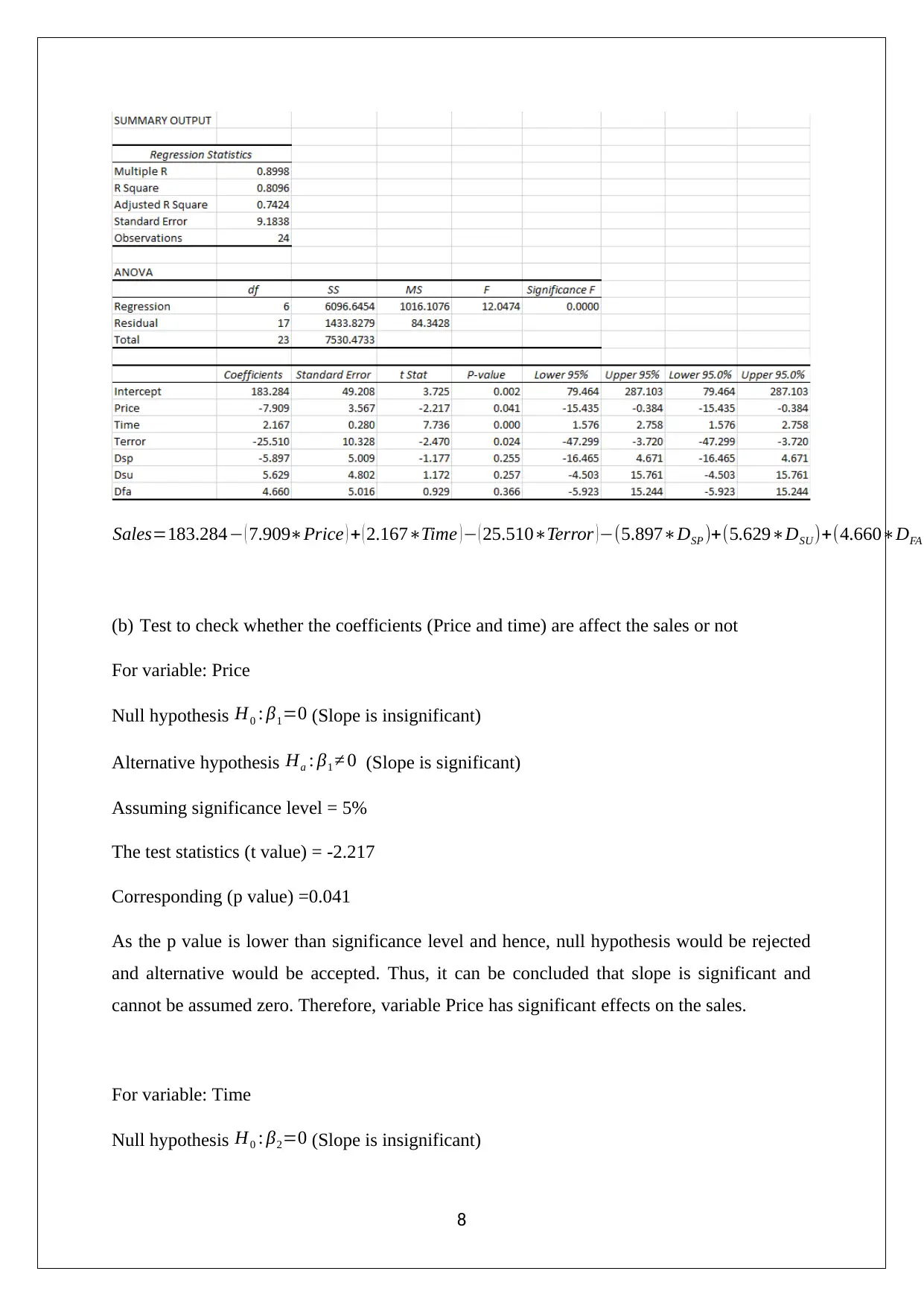
(a) Regression output
7

Sales=183.284− ( 7.909∗Price ) + ( 2.167∗Time ) − ( 25.510∗Terror ) −(5.897∗DSP )+(5.629∗DSU )+(4.660∗DFA
(b) Test to check whether the coefficients (Price and time) are affect the sales or not
For variable: Price
Null hypothesis H0 : β1=0 (Slope is insignificant)
Alternative hypothesis Ha : β1 ≠ 0 (Slope is significant)
Assuming significance level = 5%
The test statistics (t value) = -2.217
Corresponding (p value) =0.041
As the p value is lower than significance level and hence, null hypothesis would be rejected
and alternative would be accepted. Thus, it can be concluded that slope is significant and
cannot be assumed zero. Therefore, variable Price has significant effects on the sales.
For variable: Time
Null hypothesis H0 : β2=0 (Slope is insignificant)
8

Alternative hypothesis Ha : β2 ≠ 0 (Slope is significant)
Assuming significance level = 5%
The test statistics (t value) = 7.736
Corresponding (p value) =0.000
As the p value is lower than significance level and hence, null hypothesis would be rejected
and alternative would be accepted. Thus, it can be concluded that slope is significant and
cannot be assumed zero. Therefore, variable time has significant effects on the sales.
(c) Interpretation of slopes
β1 ( Price ) :The slope of price indicates that an increase in the unit price by $1 would lead to
decrease in sales by 7,909 units.
β2 ( Time ) :The slope of time indicates that an increase in the time index by one would lead to
increase in sales by 2,167 units.
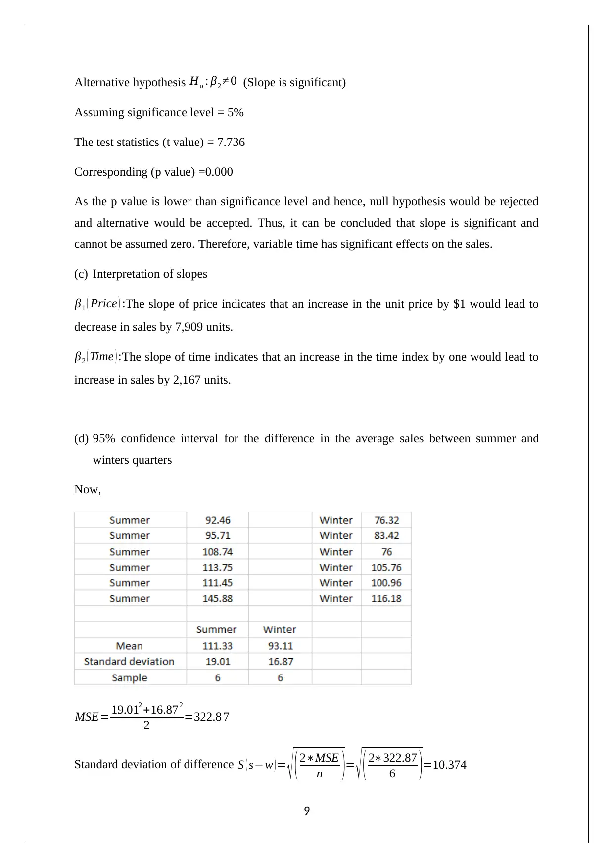
(d) 95% confidence interval for the difference in the average sales between summer and
winters quarters
Now,
MSE= 19.012 +16.872
2 =322.8 7
Standard deviation of difference S ( s−w )= √ (2∗MSE
n )= √ ( 2∗322.87
6 )=10.374
9

Mean of difference M (s-w) = 111.33 – 93.11 = 18.23
Degree of freedom = n1 +n2 -2 = 6+6-2 = 10
The t value for 95% confidence interval and 10 degree of freedom = 2.228
Now,
The lower limit of 95% confidence interval = 18.23 – (2.228*10.374) = -4.889
The Uppwe limit of 95% confidence interval = 18.23 + (2.228*10.374) = 41.339
Hence, the 95% confidence interval for the difference in the average sales between summer
and winters quarters [ -4.889 41.339].
(e) Hypothesis testing for β6 (DFA ¿
Null hypothesis H0 : β6=0
Alternative hypothesis Ha : β6>0
Assuming significance level = 5%
The test statistics (t value) = 0.929
Corresponding (p value) = 0.366
As the p value is higher than significance level and hence, null hypothesis would not be
rejected and alternative would not be accepted. Thus, it can be concluded that slope DFA
would not be higher than zero.
(f) 95% confidence interval
For variable DFA
From Regression Model
Lower limit of 95% confidence interval = -5.923
Upper limit of 95% confidence interval = 15.244
95% confidence interval = [-5.923 15.244]
10

(g) Overall significance of regression model
Null hypothesis H0 : β1=β2=β3=β4= β5 =0
Alternative hypothesis Ha :At least one of the slope coefficients is not zero.
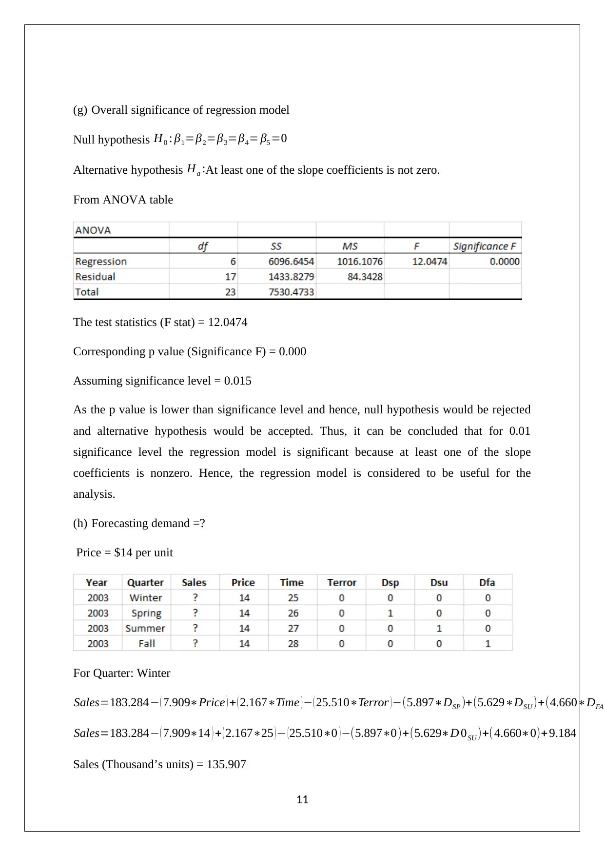
From ANOVA table
The test statistics (F stat) = 12.0474
Corresponding p value (Significance F) = 0.000
Assuming significance level = 0.015
As the p value is lower than significance level and hence, null hypothesis would be rejected
and alternative hypothesis would be accepted. Thus, it can be concluded that for 0.01
significance level the regression model is significant because at least one of the slope
coefficients is nonzero. Hence, the regression model is considered to be useful for the
analysis.
(h) Forecasting demand =?
Price = $14 per unit
For Quarter: Winter
Sales=183.284− ( 7.909∗Price ) + ( 2.167∗Time ) − ( 25.510∗Terror ) −(5.897∗DSP )+(5.629∗DSU )+(4.660∗DFA
Sales=183.284− ( 7.909∗14 ) + ( 2.167∗25 )− (25.510∗0 )−(5.897∗0)+(5.629∗D 0SU )+(4.660∗0)+ 9.184
Sales (Thousand’s units) = 135.907
11

For Quarter: Spring
Sales=183.284− ( 7.909∗Price ) + ( 2.167∗Time )− ( 25.510∗Terror )−(5.897∗DSP )+(5.629∗DSU )+(4.660∗DFA
Sales=183.284− ( 7.909∗14 ) + ( 2.167∗26 ) − ( 25.510∗0 ) −(5.897∗1)+(5.629∗D 0SU )+(4.660∗0)+9.184
Sales (Thousand’s units) = 132.176
For Quarter: Summer
Sales=183.284− ( 7.909∗Price ) + ( 2.167∗Time )− ( 25.510∗Terror )−(5.897∗DSP )+(5.629∗DSU )+(4.660∗DFA
Sales=183.284− ( 7.909∗14 ) + ( 2.167∗27 ) − ( 25.510∗0 ) −( 5.897∗0)+(5.629∗1)+(4.660∗0)+ 9.184
Sales (Thousand’s units) = 145.869
For Quarter: Fall
Sales=183.284− ( 7.909∗Price ) + ( 2.167∗Time )− ( 25.510∗Terror )−(5.897∗DSP )+(5.629∗DSU )+(4.660∗DFA
Sales=183.284− ( 7.909∗14 ) + ( 2.167∗28 )− (25.510∗0 )−(5.897∗0)+(5.629∗0)+(4.660∗1)+9.184
Sales (Thousand’s units) = 147.067
12