MBALN 603 Statistics Examination 2: Confidence Intervals & Testing

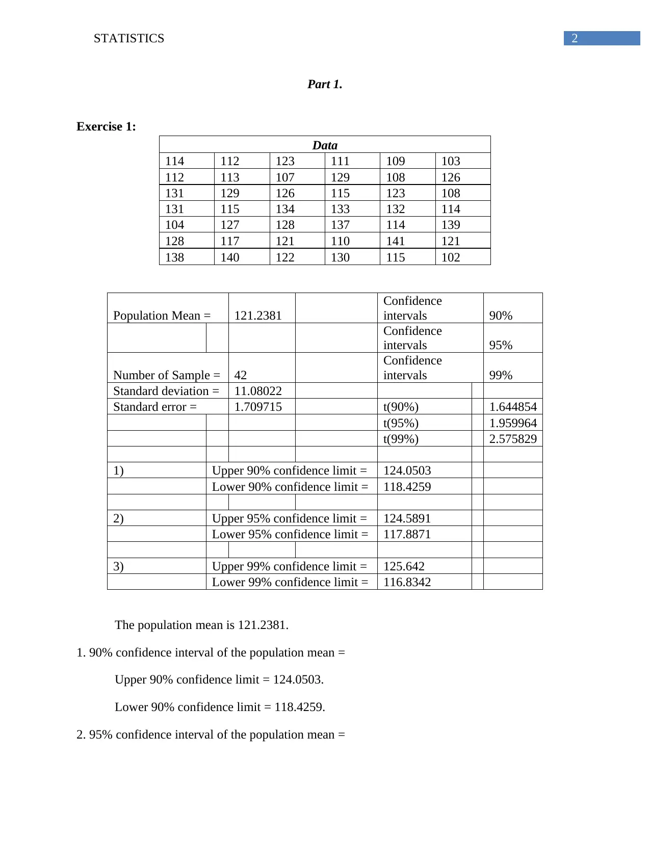
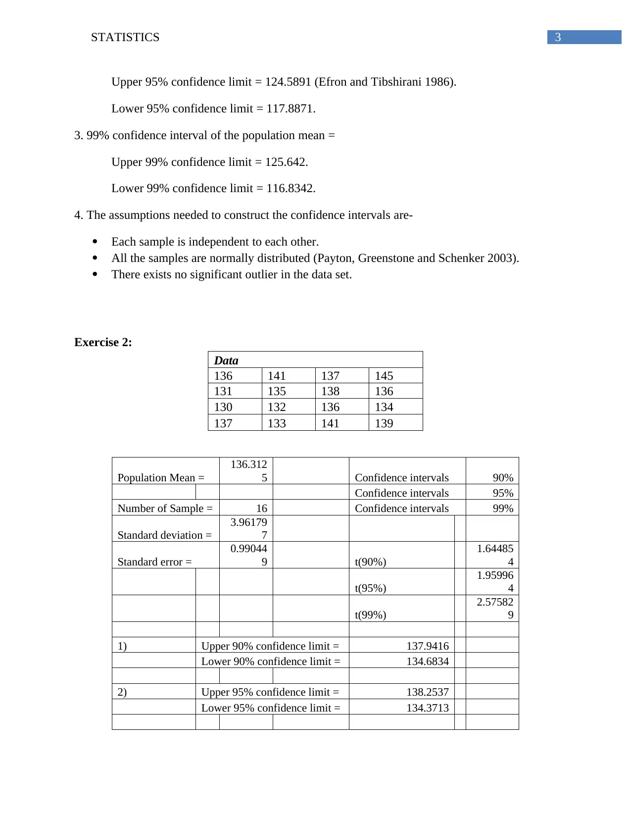
This assignment focuses on statistical analysis, including the construction and interpretation of confidence intervals for population means and hypothesis testing. Exercise 1 involves calculating 90%, 95%, and 99% confidence intervals for a given dataset, emphasizing the assumptions required for their construction, such as independence, normality, and the absence of significant outliers. Exercise 2 repeats this process with a different dataset. Exercise 3 tests the hypothesis concerning the proportions of white balls in two boxes using a two-sample proportional Z-test, determining whether the proportion in Box A is significantly greater than in Box B. Finally, Exercise 4 uses a one-way ANOVA to determine if the averages of grades from four different classes are equal, interpreting the F-statistic and p-value relative to a 5% significance level, ultimately concluding whether the null hypothesis can be rejected. The assignment includes relevant statistical references.

STATISTICS
Statistics
Name of the student:
Name of the university:
Course ID:

1STATISTICS
Table of Contents
Exercise 1:.......................................................................................................................................2
Exercise 2:.......................................................................................................................................3
Exercise 3:.......................................................................................................................................4
Exercise 4:.......................................................................................................................................6
References:......................................................................................................................................8

2STATISTICS
Part 1.
Exercise 1:
Data
114 112 123 111 109 103
112 113 107 129 108 126
131 129 126 115 123 108
131 115 134 133 132 114
104 127 128 137 114 139
128 117 121 110 141 121
138 140 122 130 115 102
Population Mean = 121.2381
Confidence
intervals 90%
Confidence
intervals 95%
Number of Sample = 42
Confidence
intervals 99%
Standard deviation = 11.08022
Standard error = 1.709715 t(90%) 1.644854
t(95%) 1.959964
t(99%) 2.575829
1) Upper 90% confidence limit = 124.0503
Lower 90% confidence limit = 118.4259
2) Upper 95% confidence limit = 124.5891
Lower 95% confidence limit = 117.8871
3) Upper 99% confidence limit = 125.642
Lower 99% confidence limit = 116.8342
The population mean is 121.2381.
1. 90% confidence interval of the population mean =
Upper 90% confidence limit = 124.0503.
Lower 90% confidence limit = 118.4259.
2. 95% confidence interval of the population mean =

3STATISTICS
Upper 95% confidence limit = 124.5891 (Efron and Tibshirani 1986).
Lower 95% confidence limit = 117.8871.
3. 99% confidence interval of the population mean =
Upper 99% confidence limit = 125.642.
Lower 99% confidence limit = 116.8342.
4. The assumptions needed to construct the confidence intervals are-
 Each sample is independent to each other.
 All the samples are normally distributed (Payton, Greenstone and Schenker 2003).
 There exists no significant outlier in the data set.
Exercise 2:
Data
136 141 137 145
131 135 138 136
130 132 136 134
137 133 141 139
Population Mean =
136.312
5 Confidence intervals 90%
Confidence intervals 95%
Number of Sample = 16 Confidence intervals 99%
Standard deviation =
3.96179
7
Standard error =
0.99044
9 t(90%)
1.64485
4
t(95%)
1.95996
4
t(99%)
2.57582
9
1) Upper 90% confidence limit = 137.9416
Lower 90% confidence limit = 134.6834
2) Upper 95% confidence limit = 138.2537
Lower 95% confidence limit = 134.3713

4STATISTICS
3) Upper 99% confidence limit = 138.8637
Lower 99% confidence limit = 133.7613
(Source: Altman and Gardner 1988)
The population mean is 136.3125.
1. 90% confidence interval of the population mean =
Upper 90% confidence limit = 137.9416.
Lower 90% confidence limit = 134.6834.
2. 95% confidence interval of the population mean =
Upper 95% confidence limit = 138.2537.
Lower 95% confidence limit = 134.3713.
3. 99% confidence interval of the population mean =
Upper 99% confidence limit = 138.8637.
Lower 99% confidence limit = 133.7613.
4. The assumptions needed to construct the confidence intervals are-
 Each sample are independent to each other (Ci 1987).
 All the samples are normally distributed.
 There exists no significant outlier in the data set.
Exercise 3:
Null hypothesis: The proportions of white balls in two boxes are equal.
Alternative
hypothesis:
The proportions of white balls in box A is greater than
box B.
Box A Box B
Total balls (n1) = 100 Total balls (n2) = 100
White balls = 52 White balls = 44
Proportion (p1) = 0.52 Proportion (p2) = 0.44
Difference in proportions (p1 - p2) 0.08

5STATISTICS
=
Total samples (n1+n2) = 200
Total white balls = 96
Total proportion (p-bar) = 0.48
Z-statistic =
1.13227
7
Level of significance
= 5%
Z-critical =
1.95996
4
Sig. = Cannot reject null hypothesis
Hypothesis:
The hypotheses are-
Null hypothesis (H0): Box A has equal proportion of white ball such as proportion of white ball
in Box B.
Alternative hypothesis (HA): Box A has higher proportion of white ball than the proportion of
white ball in Box B.
Level of significance:
The level of significance is assumed to be 5%.
Test applied:
Two sample proportional Z-test.
Calculated Z-statistic:
Z = ( p 1− p 2)
√❑ = 1.132277 (Sahai and Khurshid 1996)
(p1= proportion of white ball in box A; p2= proportion of white ball in box B; p=proportion of
white ball together in box A and box B, n1= total number of balls in box A; n2= total number of
balls in box B).
Decision-making:
1.959964>1.132277, so, Zsig.>Zcrit. Therefore, the null hypothesis could not be rejected with 95%
probability (Levine et al. 1999).
Interpretation:

6STATISTICS
Therefore, it could be interpreted that Box A has equal proportion of white ball of proportion of
white ball in Box B.
Exercise 4:
Anova: Single Factor
SUMMARY
Groups Count Sum
Averag
e
Varianc
e
Grade A 20 1445 72.25
292.407
9
Grade B 17 1164
68.4705
9
217.264
7
Grade C 15 1074 71.6
95.6857
1
Grade D 12 887
73.9166
7
238.628
8
ANOVA
Source of
Variation SS df MS F P-value F crit
Between
Groups
236.935
5 3
78.9785
1
0.36461
4
0.77877
6
2.75807
8
Within Groups 12996.5 60
216.608
4
Total
13233.4
4 63
Hypothesis:
The hypotheses are-
Null hypothesis (H0): The averages of four different grades A, B, C and D of four different
classes are equal to each other (Heiberger and Neuwirth 2009).
Alternative hypothesis (H0): There exists at least one inequality in the averages of four different
grades A, B, C and D of four different classes.
Observations:

7STATISTICS
The average of grade A is 72.25, grade B is 68.47, grade C is 71.6 and grade D is 73.92.
Test applied:
One-way ANOVA.
Level of Significance:
The level of significance is found to be 5%.
Test Statistic:
Calculated F-statistic = 0.364614 with p-value = 0.778776.
Decision-making:
As, calculated p-value is greater than the 5% level of significance, therefore, null hypothesis
could not be rejected with 95% probability (Christensen 1987). On the other hand, as Fcrit.is
greater than Fcal.(2.758078>0.364614), therefore, null hypothesis is accepted with 95% possibility
(Ross and Willson 2017).
Interpretation:
The averages of four different grades A, B, C and D of four different classes are equal to each
other.

8STATISTICS
References:
Altman, D.G. and Gardner, M.J., 1988. Statistics in Medicine: Calculating confidence intervals
for regression and correlation. British medical journal (Clinical research ed.), 296(6631),
p.1238.
Christensen, R., 1987. One-Way ANOVA. In Plane Answers to Complex Questions (pp. 57-69).
Springer, New York, NY.
Ci, B., 1987. Confidence intervals. Lancet, 1, pp.494-497.
Efron, B. and Tibshirani, R., 1986. Bootstrap methods for standard errors, confidence intervals,
and other measures of statistical accuracy. Statistical science, pp.54-75.
Heiberger, R.M. and Neuwirth, E., 2009. One-way anova. In R through excel (pp. 165-191).
Springer, New York, NY.
Levine, D.M., Berenson, M.L., Stephan, D. and Lysell, D., 1999. Statistics for managers using
Microsoft Excel (Vol. 660). Upper Saddle River, NJ: Prentice Hall.
Payton, M.E., Greenstone, M.H. and Schenker, N., 2003. Overlapping confidence intervals or
standard error intervals: what do they mean in terms of statistical significance?. Journal of Insect
Science, 3(1).
Ross, A. and Willson, V.L., 2017. One-Way Anova. In Basic and Advanced Statistical Tests (pp.
21-24). SensePublishers, Rotterdam.
Sahai, H. and Khurshid, A., 1996. Formulae and tables for the determination of sample sizes and
power in clinical trials for testing differences in proportions for the two‐sample design: a
review. Statistics in medicine, 15(1), pp.1-21.