Statistics for Financial Decisions

This assignment evaluates the market price of houses in different Australian cities over a period of 14 years. The relationship between the house prices with the Market Price, Sydney Price Index, Annual Percentage change in Price, total number of Square meters and age of the houses has been established through regression analysis.

Running Head: STATISTICS FOR FINANCIAL DECISIONS
Statistics for Financial Decisions
Name of the Student
Name of the University
Author Note

1STATISTICS FOR FINANCIAL DECISIONS
1.0 Introduction
The market price of the houses in different Australian cities has to be evaluated in this
assignment. The nature of the market prices of houses in Australia is the main interest for this
assignment over a period of 14 years is of the main interest in this assignment. In order to
understand the changes in the prices, the house price indices of the Australian States are
necessary. The house price indices of the Australian cities such as Brisbane, Sydney and
Melbourne over the 14 years from 2002 to 2016 has been provided.
Other than the house price indices for different Australian states, other factors are also
responsible for the market value of the Australian houses (Kohler and Van Der Merwe 2015).
The variables that are considered in this assignment are the annual percentage change in the
house prices, the area of the house (number of square meters) and the age of the house (in years).
The market price of the houses in Sydney has been evaluated in this assignment. Thus, the price
index of Sydney has only been considered. The results and discussion of the results have been
provided in the following section.
2.0 Results and Discussions
2.1 Relationship between Independent and Dependent Variables
In this assignment relationship between the house prices with the Market Price, Sydney
Price Index, Annual Percentage change in Price, total number of Square meters and age of the
houses has to be evaluated. Thus, market price is the dependent variable considered and the
independent variables considered are Sydney Price Index, Annual percentage change in the
prices, total number of square meters and the age of the house

2STATISTICS FOR FINANCIAL DECISIONS
Thus, at first, the nature of the relationship of each of the independent variable with the
dependent variable has been evaluated with the help of scatter plots. It can be seen from the
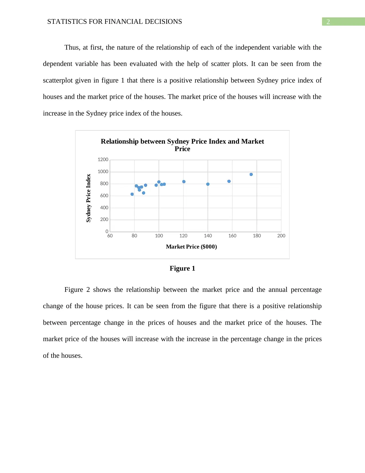
scatterplot given in figure 1 that there is a positive relationship between Sydney price index of
houses and the market price of the houses. The market price of the houses will increase with the
increase in the Sydney price index of the houses.
60 80 100 120 140 160 180 200
0
200
400
600
800
1000
1200
Relationship between Sydney Price Index and Market
Price
Market Price ($000)
Sydney Price Index
Figure 1
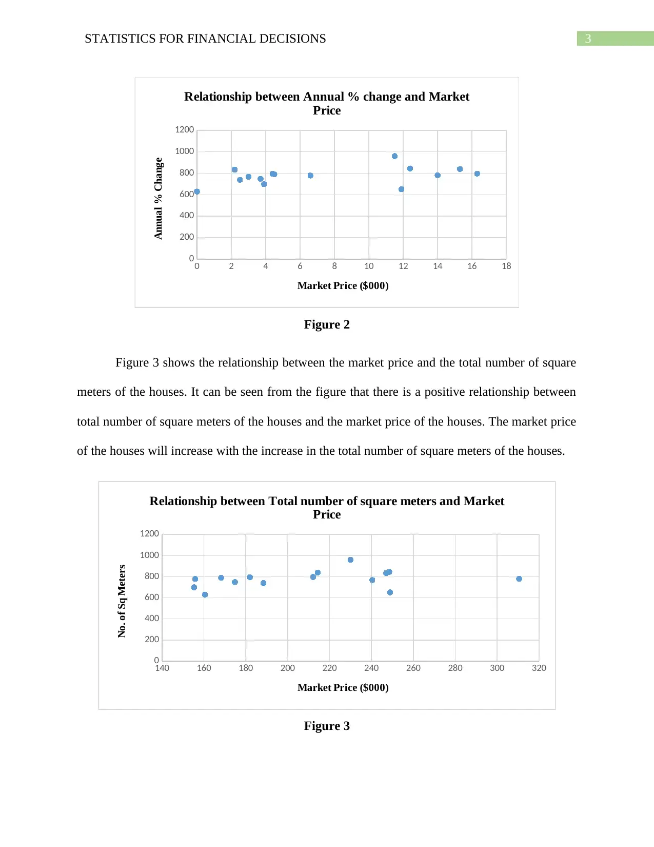
Figure 2 shows the relationship between the market price and the annual percentage
change of the house prices. It can be seen from the figure that there is a positive relationship
between percentage change in the prices of houses and the market price of the houses. The
market price of the houses will increase with the increase in the percentage change in the prices
of the houses.

3STATISTICS FOR FINANCIAL DECISIONS
0 2 4 6 8 10 12 14 16 18
0
200
400
600
800
1000
1200
Relationship between Annual % change and Market
Price
Market Price ($000)
Annual % Change
Figure 2
Figure 3 shows the relationship between the market price and the total number of square
meters of the houses. It can be seen from the figure that there is a positive relationship between
total number of square meters of the houses and the market price of the houses. The market price
of the houses will increase with the increase in the total number of square meters of the houses.
140 160 180 200 220 240 260 280 300 320
0
200
400
600
800
1000
1200
Relationship between Total number of square meters and Market
Price
Market Price ($000)
No. of Sq Meters
Figure 3

4STATISTICS FOR FINANCIAL DECISIONS
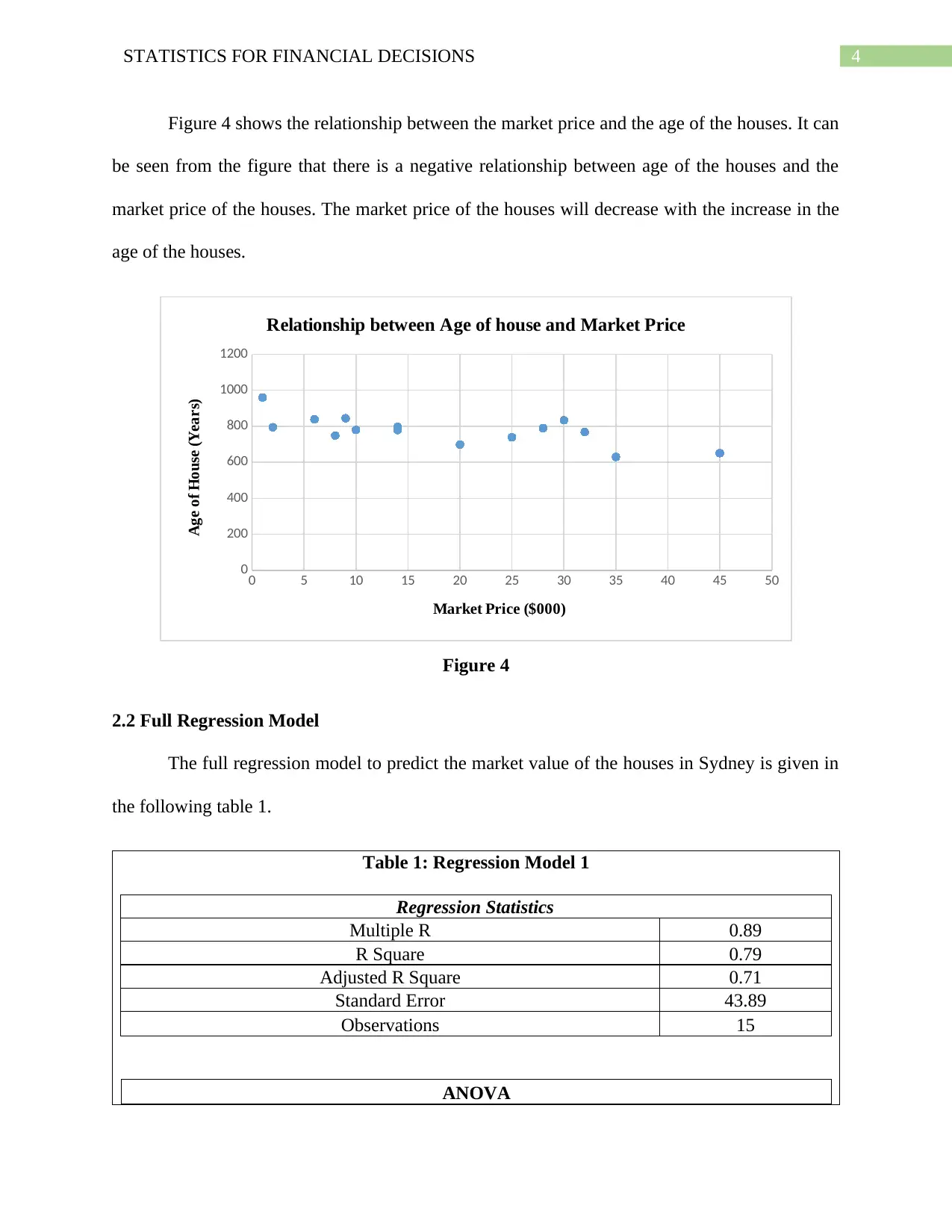
Figure 4 shows the relationship between the market price and the age of the houses. It can
be seen from the figure that there is a negative relationship between age of the houses and the
market price of the houses. The market price of the houses will decrease with the increase in the
age of the houses.
0 5 10 15 20 25 30 35 40 45 50
0
200
400
600
800
1000
1200
Relationship between Age of house and Market Price
Market Price ($000)
Age of House (Years)
Figure 4
2.2 Full Regression Model
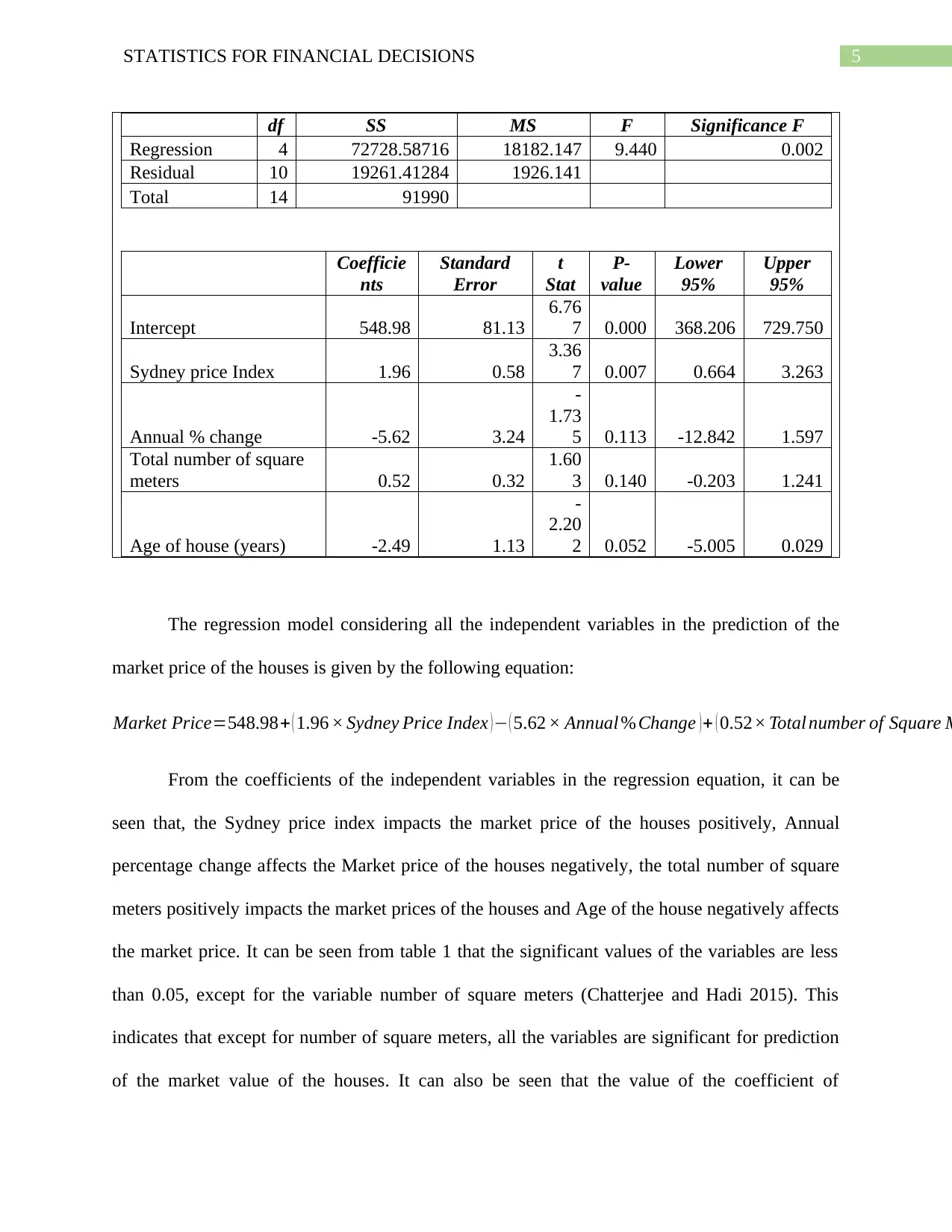
The full regression model to predict the market value of the houses in Sydney is given in
the following table 1.
Table 1: Regression Model 1
Regression Statistics
Multiple R 0.89
R Square 0.79
Adjusted R Square 0.71
Standard Error 43.89
Observations 15
ANOVA

5STATISTICS FOR FINANCIAL DECISIONS
df SS MS F Significance F
Regression 4 72728.58716 18182.147 9.440 0.002
Residual 10 19261.41284 1926.141
Total 14 91990
Coefficie
nts
Standard
Error
t
Stat
P-
value
Lower
95%
Upper
95%
Intercept 548.98 81.13
6.76
7 0.000 368.206 729.750
Sydney price Index 1.96 0.58
3.36
7 0.007 0.664 3.263
Annual % change -5.62 3.24
-
1.73
5 0.113 -12.842 1.597
Total number of square
meters 0.52 0.32
1.60
3 0.140 -0.203 1.241
Age of house (years) -2.49 1.13
-
2.20
2 0.052 -5.005 0.029
The regression model considering all the independent variables in the prediction of the
market price of the houses is given by the following equation:
Market Price=548.98+ ( 1.96 × Sydney Price Index ) − ( 5.62 × Annual % Change ) + ( 0.52× Total number of Square M
From the coefficients of the independent variables in the regression equation, it can be
seen that, the Sydney price index impacts the market price of the houses positively, Annual
percentage change affects the Market price of the houses negatively, the total number of square
meters positively impacts the market prices of the houses and Age of the house negatively affects
the market price. It can be seen from table 1 that the significant values of the variables are less
than 0.05, except for the variable number of square meters (Chatterjee and Hadi 2015). This
indicates that except for number of square meters, all the variables are significant for prediction
of the market value of the houses. It can also be seen that the value of the coefficient of

6STATISTICS FOR FINANCIAL DECISIONS
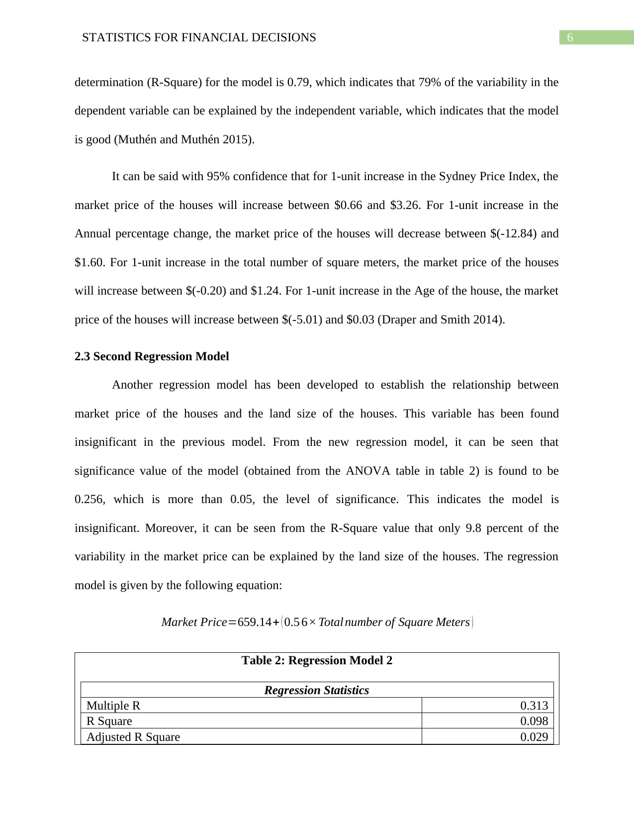
determination (R-Square) for the model is 0.79, which indicates that 79% of the variability in the
dependent variable can be explained by the independent variable, which indicates that the model
is good (Muthén and Muthén 2015).
It can be said with 95% confidence that for 1-unit increase in the Sydney Price Index, the
market price of the houses will increase between $0.66 and $3.26. For 1-unit increase in the
Annual percentage change, the market price of the houses will decrease between $(-12.84) and
$1.60. For 1-unit increase in the total number of square meters, the market price of the houses
will increase between $(-0.20) and $1.24. For 1-unit increase in the Age of the house, the market
price of the houses will increase between $(-5.01) and $0.03 (Draper and Smith 2014).
2.3 Second Regression Model
Another regression model has been developed to establish the relationship between
market price of the houses and the land size of the houses. This variable has been found
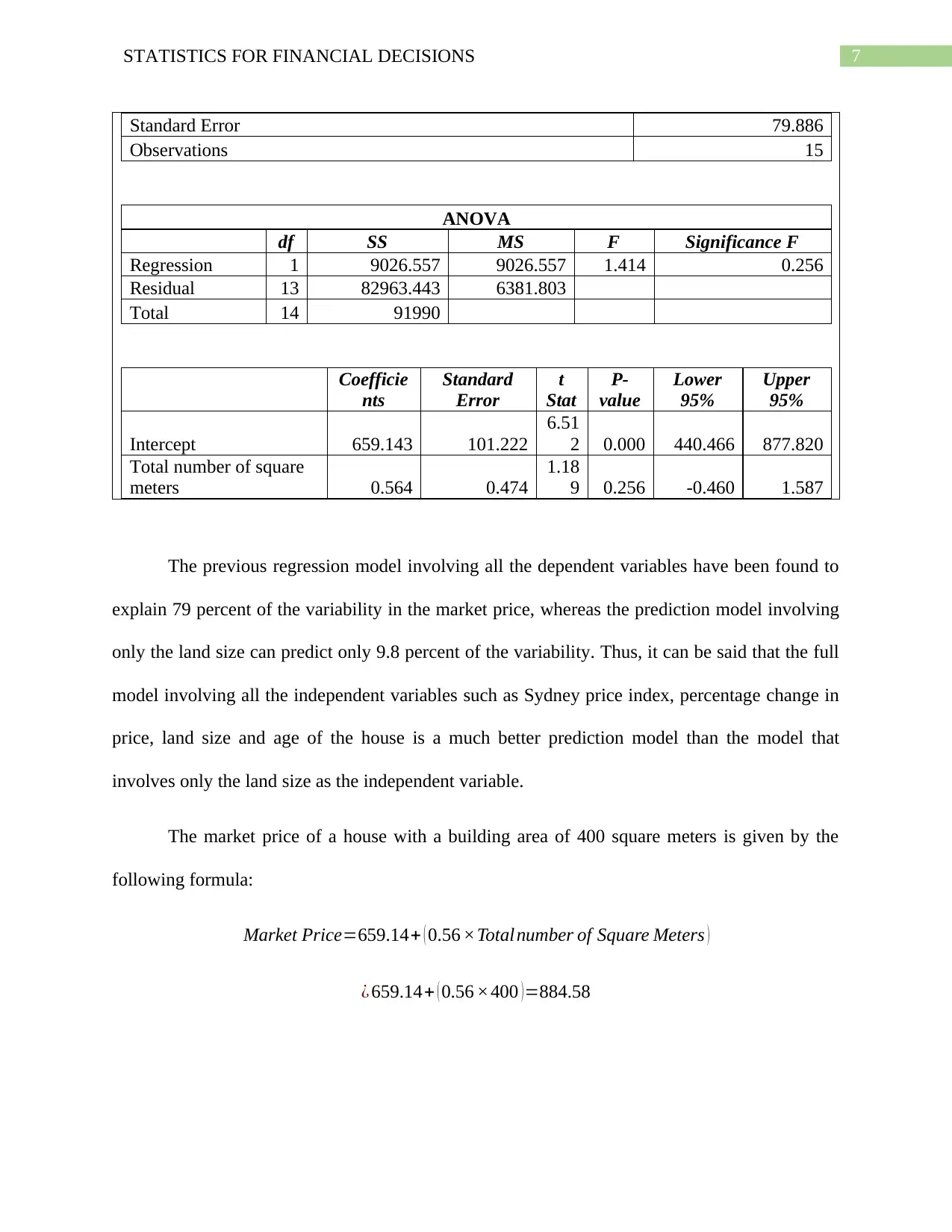
insignificant in the previous model. From the new regression model, it can be seen that
significance value of the model (obtained from the ANOVA table in table 2) is found to be
0.256, which is more than 0.05, the level of significance. This indicates the model is
insignificant. Moreover, it can be seen from the R-Square value that only 9.8 percent of the
variability in the market price can be explained by the land size of the houses. The regression
model is given by the following equation:
Market Price=659.14+ ( 0.5 6× Total number of Square Meters )
Table 2: Regression Model 2
Regression Statistics
Multiple R 0.313
R Square 0.098
Adjusted R Square 0.029

7STATISTICS FOR FINANCIAL DECISIONS
Standard Error 79.886
Observations 15
ANOVA
df SS MS F Significance F
Regression 1 9026.557 9026.557 1.414 0.256
Residual 13 82963.443 6381.803
Total 14 91990
Coefficie
nts
Standard
Error
t
Stat
P-
value
Lower
95%
Upper
95%
Intercept 659.143 101.222
6.51
2 0.000 440.466 877.820
Total number of square
meters 0.564 0.474
1.18
9 0.256 -0.460 1.587
The previous regression model involving all the dependent variables have been found to
explain 79 percent of the variability in the market price, whereas the prediction model involving
only the land size can predict only 9.8 percent of the variability. Thus, it can be said that the full
model involving all the independent variables such as Sydney price index, percentage change in
price, land size and age of the house is a much better prediction model than the model that
involves only the land size as the independent variable.
The market price of a house with a building area of 400 square meters is given by the
following formula:
Market Price=659.14+ ( 0.56 ×Total number of Square Meters )
¿ 659.14+ ( 0.56 ×400 )=884.58

8STATISTICS FOR FINANCIAL DECISIONS
3.0 Conclusion
Analysis of the property data over 14 years have been performed. Relationship between
market price of the houses in Sydney with the Sydney price index, percentage change in the
prices from previous year, land size and age of the houses have been established. It has been
observed that Sydney price index and land size has a positive relationship with market price and
percentage change in price and age of the house has a negative relationship. Moreover, land size
has been found to be insignificant. The prediction model involving all the four dependent
variables have been observed to be a much better model that the one involving only the land size.

9STATISTICS FOR FINANCIAL DECISIONS
References
Chatterjee, S. and Hadi, A.S., 2015. Regression analysis by example. John Wiley & Sons.
Draper, N.R. and Smith, H., 2014. Applied regression analysis (Vol. 326). John Wiley & Sons.
Kohler, M. and Van Der Merwe, M., 2015. Long-run trends in housing price growth. Reserve
Bank Bulletin, pp.21-30.
Muthén, L.K. and Muthén, B., 2015. Mplus. The comprehensive modelling program for applied
researchers: user’s guide, 5.