Statistics for Financial Decisions Using Excel

Running head: STATISTICS FOR FINANCIAL DECISIONS
1
Statistics for Financial Decisions Using Excel
Name of Author
Class Name
Name of School

STATISTICS FOR FINANCIAL DECISIONS 2
Abstract
The requirement of this assignment is the analysis of financial data using excel to help
make appropriate financial decisions. In the process of analysis, a regression model is supposed
to be developed. The regression model by chance is supposed to have one dependent variable
and four independent variables. From the idea of regression models, a model with more than one
independent variable is a multiple linear regression model. Hence what we actually are expected
to have is a multiple linear regression model. The actual model will look something like;
Y = β0 + β1 X1 + β2 X2 + β3 X3 + β4 X4 + ε (Harrell, 2015). Where Y is treated as the value of the
dependent variable, β0 is treated as the regression constant, β1 partial regression coefficients of
the first variable, β2 partial regression coefficient of the second variable, β3 partial regression
coefficient of the third variable, β4 partial regression coefficient of the fourth coefficient and ε is
treated as the error term.
Introduction
In this section of one of them, a statement that we are supposed to do is the rationale of
the model that we have developed via analysis. Our model is a multiple linear regression which
basically has got four independent variables and one dependent variable, unlike simple linear
regression which has one independent variable. Multiple linear regressions, our model, is
basically tracing its foundation from the correlation analysis. The first independent variable, in
analysis, explains the most of variance whereas the second independent variable explains the
second most of the variance and so on. In summary, the independent variables, help in analysis
to explain a proportional percentage of the variance of the dependent variable. Our model
replicates the identification related to important independent variables (Riley, Jackson, Salanti,

STATISTICS FOR FINANCIAL DECISIONS 3
Burke, Price, Kirkham & White, 2017). One disadvantage is that the model replicates error as
well. As it is known though, there is no model that is always perfect in the analysis (Akinwande,
Dikko & Samson, 2015).
The sample size of the model developed is fifteen cases for each predictor. This means
that for each independent variable there are actually fifteen observations. This is evident even
when you look at the multiple linear regression results ( Bretz, Hothorn & Westfall, 2016).
The dependent variable is the market price with a unit measurement of US Dollars,
something that is supposed to be determined by the model. The independent variables are;
Sydney price index, annual % change measured in percentage, the total number of square meters
measured in square meters and age of house measured in years.
Plotting
0 50 100 150 200 250 300 350 400
0
200
400
600
800
1000
1200
Age of house (years) Total number of square meters
Annual % change Sydney price Index Figure 1
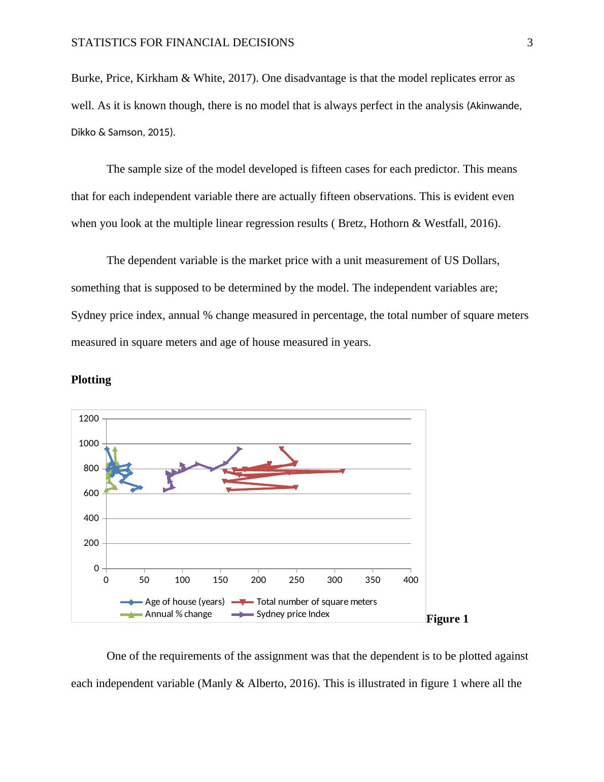
One of the requirements of the assignment was that the dependent is to be plotted against
each independent variable (Manly & Alberto, 2016). This is illustrated in figure 1 where all the

STATISTICS FOR FINANCIAL DECISIONS 4
plots for the respective variables are made. The variable; the age of house ranges from 0 to a
maximum of 45 hence the clustering to the extreme left. The actual data values when plotted will
produce a curve that crosses itself more than once. The total number of square meters being a
complete larger set of values, you find that the curve is out farther in the graph. It too has
crossing points on itself. Sydney price index keeps on rising, but the percentage change rises and
drops with it being at the extreme left as the changes are minimal but also produces a curve that
crosses itself (Mirman, 2017).
Full Model
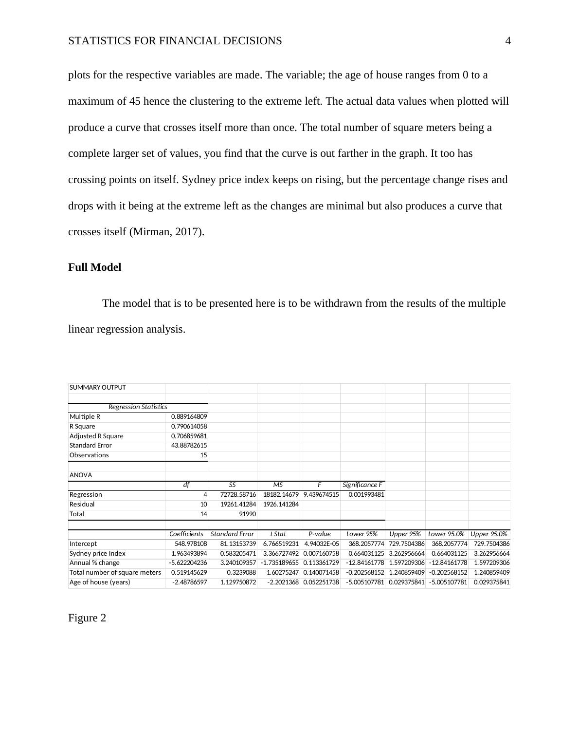
The model that is to be presented here is to be withdrawn from the results of the multiple
linear regression analysis.
SUMMARY OUTPUT
Regression Statistics
Multiple R 0.889164809
R Square 0.790614058
Adjusted R Square 0.706859681
Standard Error 43.88782615
Observations 15
ANOVA
df
SS
MS
F Significance F
Regression 4 72728.58716 18182.14679 9.439674515 0.001993481
Residual 10 19261.41284 1926.141284
Total 14 91990
Coefficients Standard Error t Stat P-value Lower 95% Upper 95% Lower 95.0% Upper 95.0%
Intercept 548.978108 81.13153739 6.766519231 4.94032E-05 368.2057774 729.7504386 368.2057774 729.7504386
Sydney price Index 1.963493894 0.583205471 3.366727492 0.007160758 0.664031125 3.262956664 0.664031125 3.262956664
Annual % change -5.622204236 3.240109357 -1.735189655 0.113361729 -12.84161778 1.597209306 -12.84161778 1.597209306
Total number of square meters 0.519145629 0.3239088 1.60275247 0.140071458 -0.202568152 1.240859409 -0.202568152 1.240859409
Age of house (years) -2.48786597 1.129750872 -2.2021368 0.052251738 -5.005107781 0.029375841 -5.005107781 0.029375841
Figure 2