Data Analysis Report of Australian Road Transport Crash Fatalities

This data analysis report analyzes the Australian road transport crash fatalities from 2010 to 2018. It includes one-variable and two-variable analysis, linear regression, and clustering.

Table of Contents
Data analysis report of the Australian road transport crash fatalities from 2010 to 2018...............2
Introduction................................................................................................................................................2
Authorization and purpose...................................................................................................................2
Limitations..............................................................................................................................................2
Scope.....................................................................................................................................................2
Methodology..............................................................................................................................................3
Data setup.................................................................................................................................................3
Exploratory data analysis.........................................................................................................................3
One variable analysis...........................................................................................................................3
One variable analysis 1........................................................................................................................3
One variable analysis 2........................................................................................................................4
One variable analysis 3........................................................................................................................5
Two-variable analysis...............................................................................................................................6
Linear regression......................................................................................................................................7
Clustering....................................................................................................................................................9
Brief explanation of k-means and clustering...........................................................................................9
Clustering analysis...................................................................................................................................9
Analysis:.....................................................................................................................................................10
Conclusion...............................................................................................................................................11
Reflections...............................................................................................................................................11
References..............................................................................................................................................11

Data analysis report of the Australian road transport crash fatalities
from 2010 to 2018
Introduction
Authorization and purpose
This data analysis report has been assembled to find trends in the Australian road transport
crash fatalities from 2010 to 2018. There are no specific achievable goals set out, but anything
found to be interesting or significant will be critically analyzed to assist other researchers,
business representatives and government agencies.
Limitations
The Australian road transport crash fatalities from 2010 to 2018 will be analyzed. The dataset
from” (https://data.gov.au/data/dataset/australian-road-deaths-database )” will be the only
data that is processed and analyzed.
Scope
Data from” (https://data.gov.au/data/dataset/australian-road-deaths-database )” will be setup
and pre-processed. Three, one-variable analysis will be performed, followed by two, two-
variable analysis. A graph will be provided with each individual analysis. Clustering and k-means
will be briefly explained and a clustering analysis to group certain states will be performed.
Linear regression will be briefly explained and two linear regression analyzes will be executed,
with both models to be plotted.

Methodology
Research for the report has been gathered from a csv data spreadsheet from
“(https://data.gov.au/data/dataset/australian-road-deaths-database )” . All references have
been gathered from journal articles from the USC library database.
Data setup
Before the data is loaded into R, the raw “road transport 1.xlsx” file should be pre-processed.
Many fields are left unrecorded and this will make cutting these rows out easier in R. Now the
collected dataset under the name of “road transport 1.xlsx” must be loaded into the
workspace. In R, by using the command getwd () the location of the R workspace can be found.
> getwd()
[1] "C:/Users/JARO/Documents"
Now that the location of the workspace is confirmed “road transport 1.xlsx” can be placed in
the work space location. Considering that the raw data is an excel workbook file (.xlsx) and not
a text file, the built in xlsx reader can be utilized to read the file information into the variable
“data”.
road_transport_1 <- read_excel("C:/Users/JARO/Downloads/road transport 1.xlsx")
Library “cluster” is loaded for a visualization of clusters.
library(cluster)
The data is split into annual values shared throughout all the series. Because of this, subplots
will have to be generated to separate the different series into categories. The data is now ready
for analysis.
Exploratory data analysis
One variable analysis
One variable analysis 1
> boxplot(road_transport_1$`Speed Limit`,ylab="Speed Limit",main="Boxplot of Speed Limit")

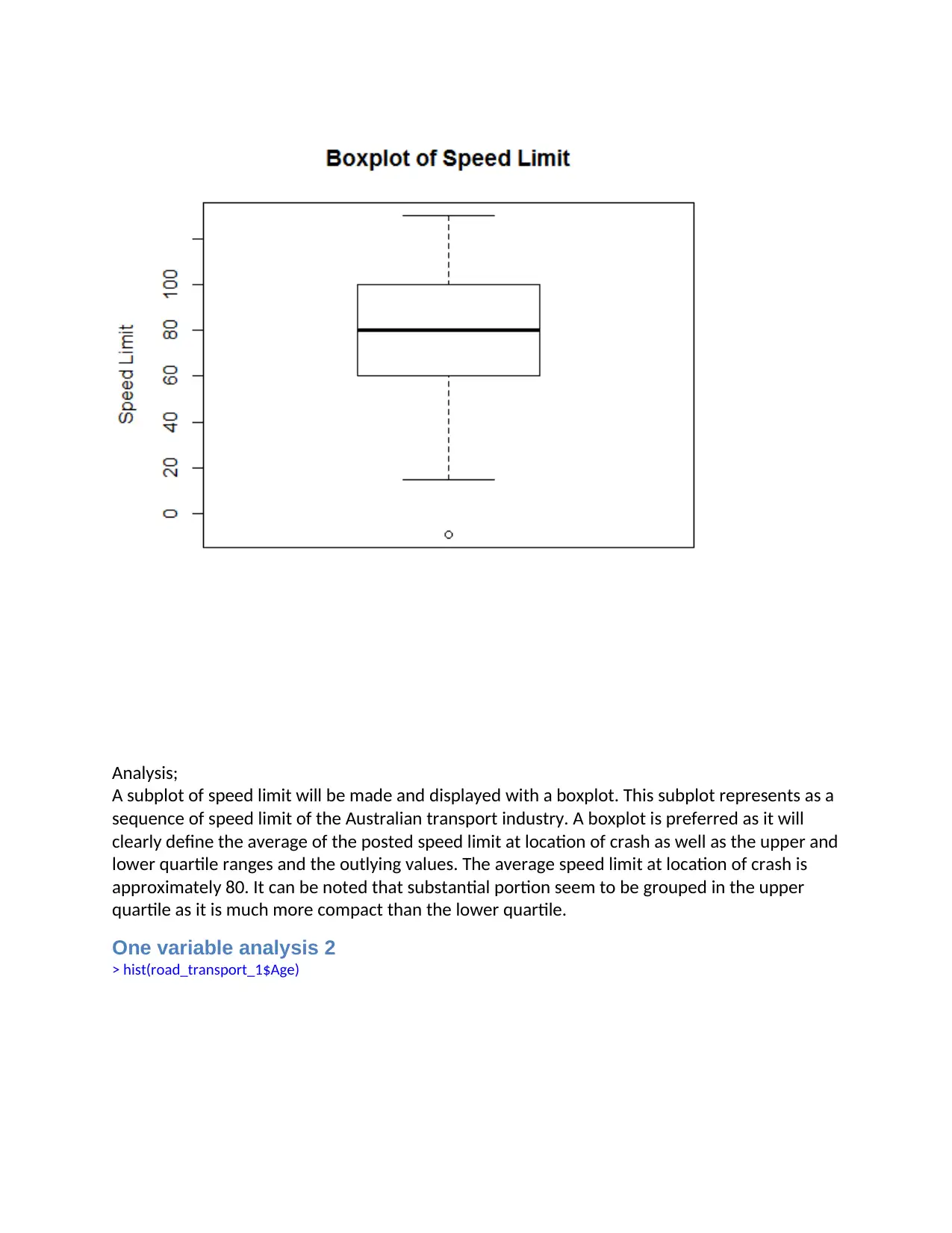
Analysis;
A subplot of speed limit will be made and displayed with a boxplot. This subplot represents as a
sequence of speed limit of the Australian transport industry. A boxplot is preferred as it will
clearly define the average of the posted speed limit at location of crash as well as the upper and
lower quartile ranges and the outlying values. The average speed limit at location of crash is
approximately 80. It can be noted that substantial portion seem to be grouped in the upper
quartile as it is much more compact than the lower quartile.
One variable analysis 2
> hist(road_transport_1$Age)

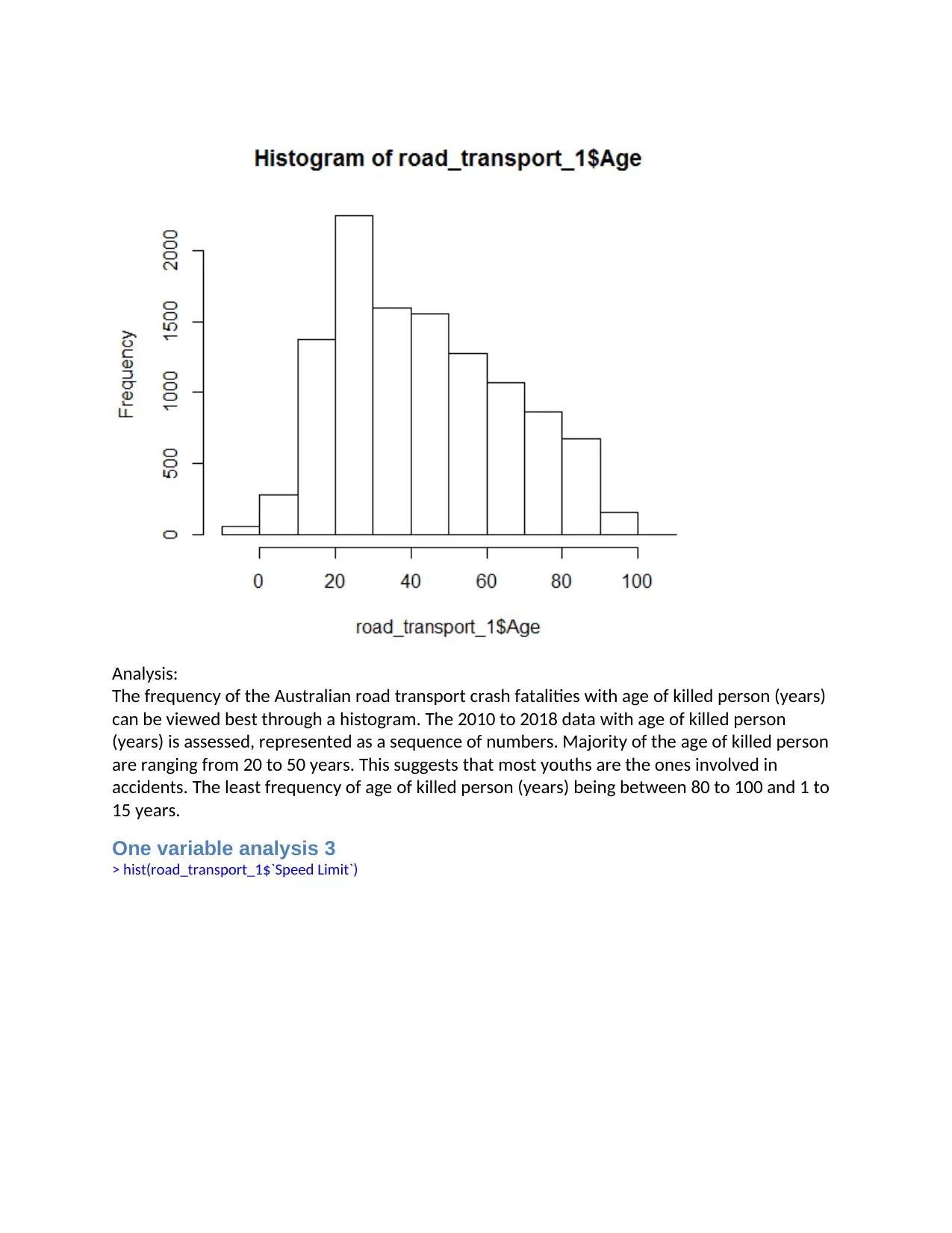
Analysis:
The frequency of the Australian road transport crash fatalities with age of killed person (years)
can be viewed best through a histogram. The 2010 to 2018 data with age of killed person
(years) is assessed, represented as a sequence of numbers. Majority of the age of killed person
are ranging from 20 to 50 years. This suggests that most youths are the ones involved in
accidents. The least frequency of age of killed person (years) being between 80 to 100 and 1 to
15 years.
One variable analysis 3
> hist(road_transport_1$`Speed Limit`)

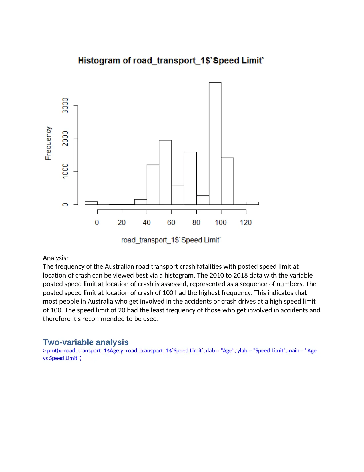
Analysis:
The frequency of the Australian road transport crash fatalities with posted speed limit at
location of crash can be viewed best via a histogram. The 2010 to 2018 data with the variable
posted speed limit at location of crash is assessed, represented as a sequence of numbers. The
posted speed limit at location of crash of 100 had the highest frequency. This indicates that
most people in Australia who get involved in the accidents or crash drives at a high speed limit
of 100. The speed limit of 20 had the least frequency of those who get involved in accidents and
therefore it’s recommended to be used.
Two-variable analysis
> plot(x=road_transport_1$Age,y=road_transport_1$`Speed Limit`,xlab = "Age", ylab = "Speed Limit",main = "Age
vs Speed Limit")

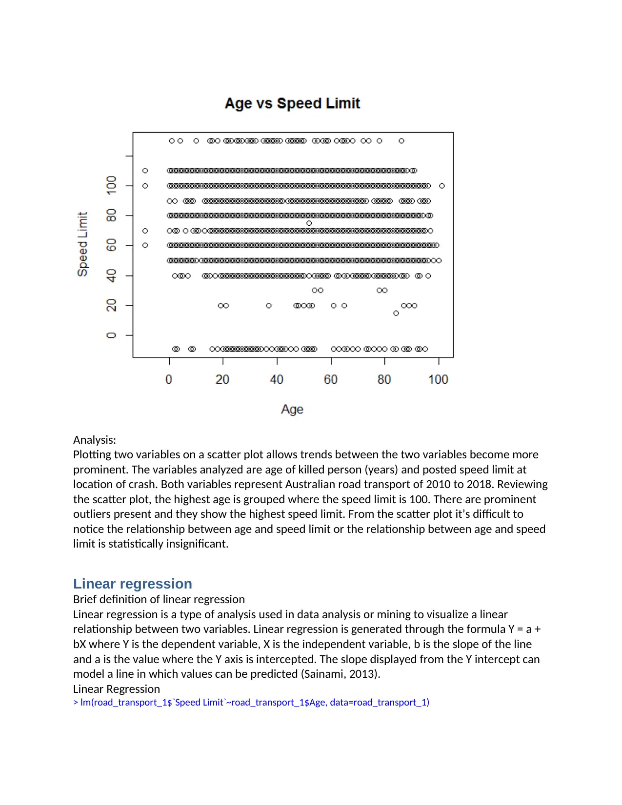
Analysis:
Plotting two variables on a scatter plot allows trends between the two variables become more
prominent. The variables analyzed are age of killed person (years) and posted speed limit at
location of crash. Both variables represent Australian road transport of 2010 to 2018. Reviewing
the scatter plot, the highest age is grouped where the speed limit is 100. There are prominent
outliers present and they show the highest speed limit. From the scatter plot it’s difficult to
notice the relationship between age and speed limit or the relationship between age and speed
limit is statistically insignificant.
Linear regression
Brief definition of linear regression
Linear regression is a type of analysis used in data analysis or mining to visualize a linear
relationship between two variables. Linear regression is generated through the formula Y = a +
bX where Y is the dependent variable, X is the independent variable, b is the slope of the line
and a is the value where the Y axis is intercepted. The slope displayed from the Y intercept can
model a line in which values can be predicted (Sainami, 2013).
Linear Regression
> lm(road_transport_1$`Speed Limit`~road_transport_1$Age, data=road_transport_1)

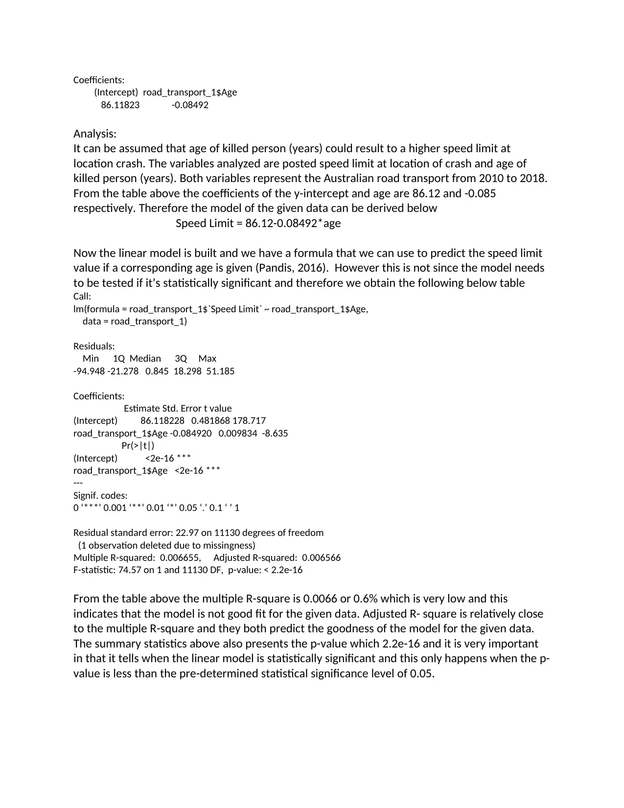
Coefficients:
(Intercept) road_transport_1$Age
86.11823 -0.08492
Analysis:
It can be assumed that age of killed person (years) could result to a higher speed limit at
location crash. The variables analyzed are posted speed limit at location of crash and age of
killed person (years). Both variables represent the Australian road transport from 2010 to 2018.
From the table above the coefficients of the y-intercept and age are 86.12 and -0.085
respectively. Therefore the model of the given data can be derived below
Speed Limit = 86.12-0.08492*age
Now the linear model is built and we have a formula that we can use to predict the speed limit
value if a corresponding age is given (Pandis, 2016). However this is not since the model needs
to be tested if it’s statistically significant and therefore we obtain the following below table
Call:
lm(formula = road_transport_1$`Speed Limit` ~ road_transport_1$Age,
data = road_transport_1)
Residuals:
Min 1Q Median 3Q Max
-94.948 -21.278 0.845 18.298 51.185
Coefficients:
Estimate Std. Error t value
(Intercept) 86.118228 0.481868 178.717
road_transport_1$Age -0.084920 0.009834 -8.635
Pr(>|t|)
(Intercept) <2e-16 ***
road_transport_1$Age <2e-16 ***
---
Signif. codes:
0 ‘***’ 0.001 ‘**’ 0.01 ‘*’ 0.05 ‘.’ 0.1 ‘ ’ 1
Residual standard error: 22.97 on 11130 degrees of freedom
(1 observation deleted due to missingness)
Multiple R-squared: 0.006655, Adjusted R-squared: 0.006566
F-statistic: 74.57 on 1 and 11130 DF, p-value: < 2.2e-16
From the table above the multiple R-square is 0.0066 or 0.6% which is very low and this
indicates that the model is not good fit for the given data. Adjusted R- square is relatively close
to the multiple R-square and they both predict the goodness of the model for the given data.
The summary statistics above also presents the p-value which 2.2e-16 and it is very important
in that it tells when the linear model is statistically significant and this only happens when the p-
value is less than the pre-determined statistical significance level of 0.05.

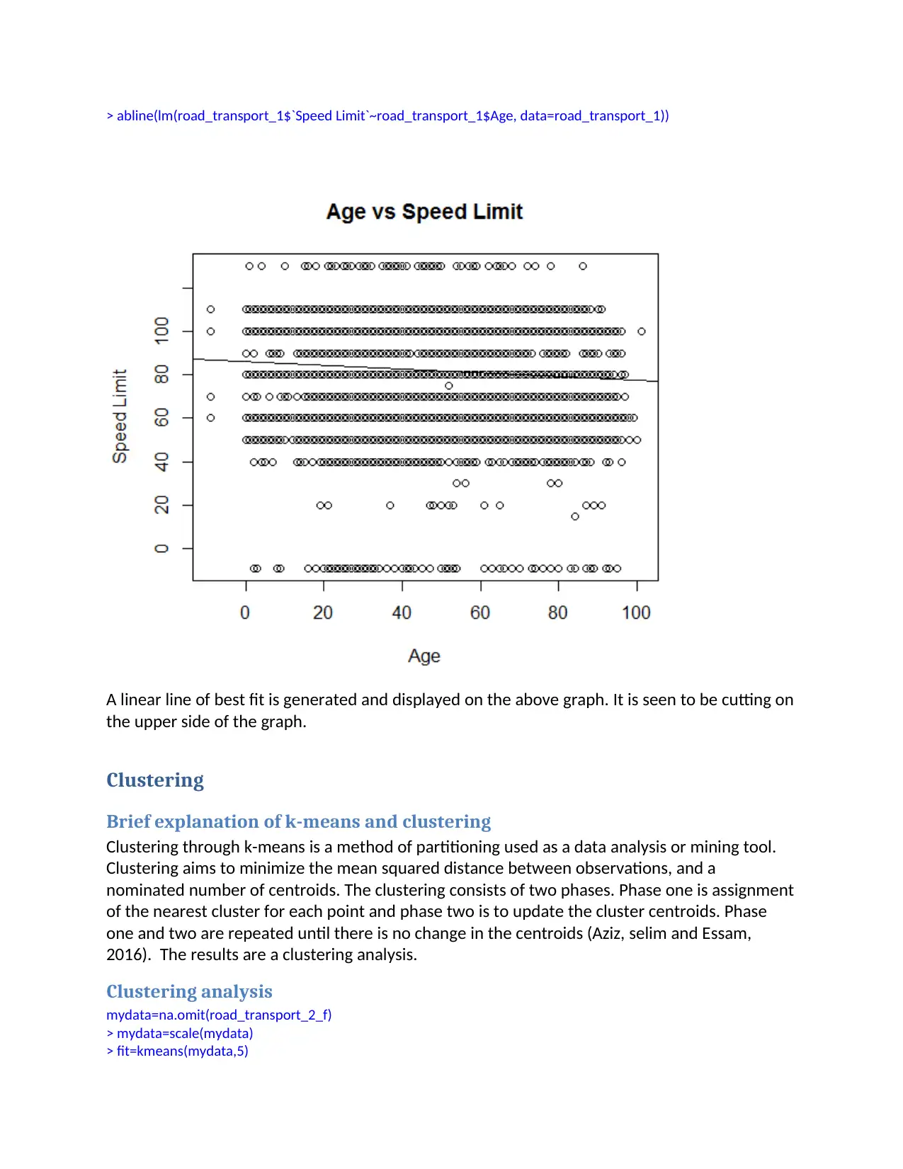
> abline(lm(road_transport_1$`Speed Limit`~road_transport_1$Age, data=road_transport_1))
A linear line of best fit is generated and displayed on the above graph. It is seen to be cutting on
the upper side of the graph.
Clustering
Brief explanation of k-means and clustering
Clustering through k-means is a method of partitioning used as a data analysis or mining tool.
Clustering aims to minimize the mean squared distance between observations, and a
nominated number of centroids. The clustering consists of two phases. Phase one is assignment
of the nearest cluster for each point and phase two is to update the cluster centroids. Phase
one and two are repeated until there is no change in the centroids (Aziz, selim and Essam,
2016). The results are a clustering analysis.
Clustering analysis
mydata=na.omit(road_transport_2_f)
> mydata=scale(mydata)
> fit=kmeans(mydata,5)

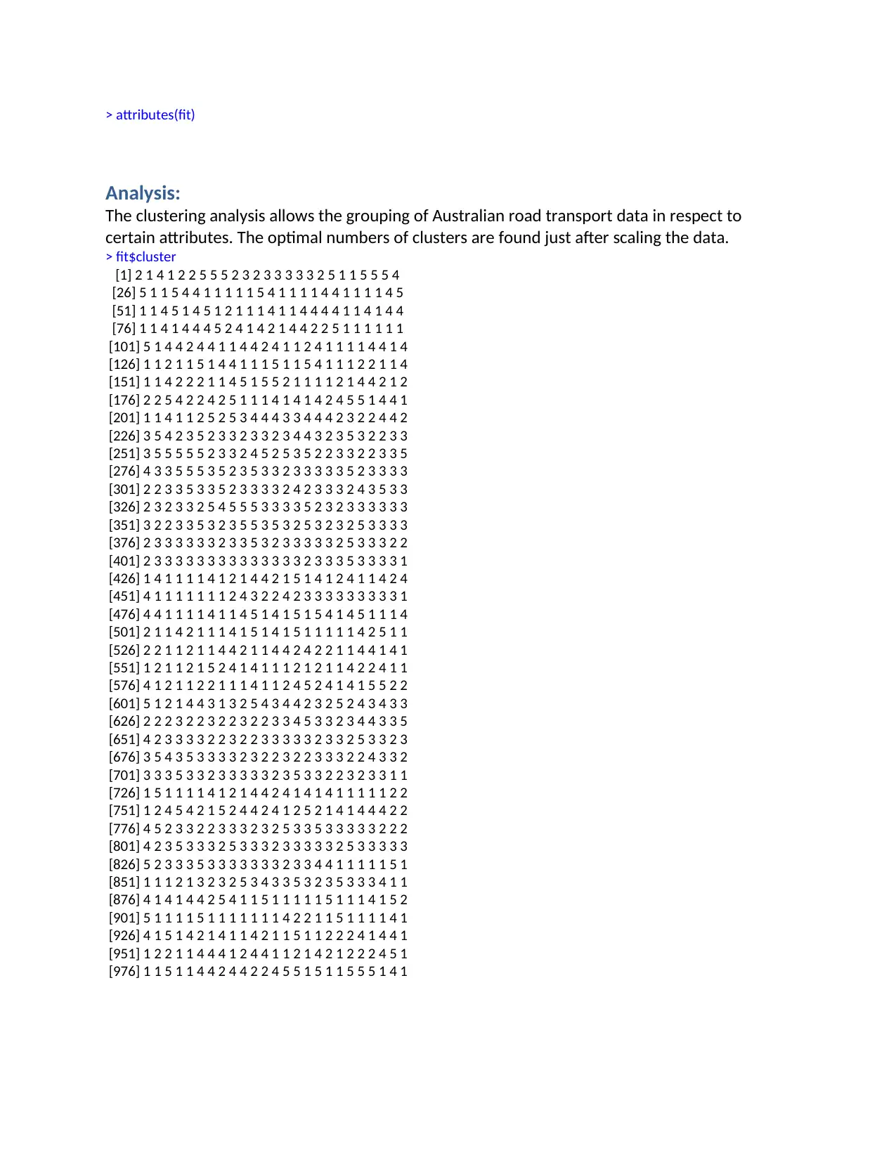
> attributes(fit)
Analysis:
The clustering analysis allows the grouping of Australian road transport data in respect to
certain attributes. The optimal numbers of clusters are found just after scaling the data.
> fit$cluster
[1] 2 1 4 1 2 2 5 5 5 2 3 2 3 3 3 3 3 2 5 1 1 5 5 5 4
[26] 5 1 1 5 4 4 1 1 1 1 1 5 4 1 1 1 1 4 4 1 1 1 1 4 5
[51] 1 1 4 5 1 4 5 1 2 1 1 1 4 1 1 4 4 4 4 1 1 4 1 4 4
[76] 1 1 4 1 4 4 4 5 2 4 1 4 2 1 4 4 2 2 5 1 1 1 1 1 1
[101] 5 1 4 4 2 4 4 1 1 4 4 2 4 1 1 2 4 1 1 1 1 4 4 1 4
[126] 1 1 2 1 1 5 1 4 4 1 1 1 5 1 1 5 4 1 1 1 2 2 1 1 4
[151] 1 1 4 2 2 2 1 1 4 5 1 5 5 2 1 1 1 1 2 1 4 4 2 1 2
[176] 2 2 5 4 2 2 4 2 5 1 1 1 4 1 4 1 4 2 4 5 5 1 4 4 1
[201] 1 1 4 1 1 2 5 2 5 3 4 4 4 3 3 4 4 4 2 3 2 2 4 4 2
[226] 3 5 4 2 3 5 2 3 3 2 3 3 2 3 4 4 3 2 3 5 3 2 2 3 3
[251] 3 5 5 5 5 5 2 3 3 2 4 5 2 5 3 5 2 2 3 3 2 2 3 3 5
[276] 4 3 3 5 5 5 3 5 2 3 5 3 3 2 3 3 3 3 3 5 2 3 3 3 3
[301] 2 2 3 3 5 3 3 5 2 3 3 3 3 2 4 2 3 3 3 2 4 3 5 3 3
[326] 2 3 2 3 3 2 5 4 5 5 5 3 3 3 3 5 2 3 2 3 3 3 3 3 3
[351] 3 2 2 3 3 5 3 2 3 5 5 3 5 3 2 5 3 2 3 2 5 3 3 3 3
[376] 2 3 3 3 3 3 3 2 3 3 5 3 2 3 3 3 3 3 2 5 3 3 3 2 2
[401] 2 3 3 3 3 3 3 3 3 3 3 3 3 3 3 2 3 3 3 5 3 3 3 3 1
[426] 1 4 1 1 1 1 4 1 2 1 4 4 2 1 5 1 4 1 2 4 1 1 4 2 4
[451] 4 1 1 1 1 1 1 1 2 4 3 2 2 4 2 3 3 3 3 3 3 3 3 3 1
[476] 4 4 1 1 1 1 4 1 1 4 5 1 4 1 5 1 5 4 1 4 5 1 1 1 4
[501] 2 1 1 4 2 1 1 1 4 1 5 1 4 1 5 1 1 1 1 1 4 2 5 1 1
[526] 2 2 1 1 2 1 1 4 4 2 1 1 4 4 2 4 2 2 1 1 4 4 1 4 1
[551] 1 2 1 1 2 1 5 2 4 1 4 1 1 1 2 1 2 1 1 4 2 2 4 1 1
[576] 4 1 2 1 1 2 2 1 1 1 4 1 1 2 4 5 2 4 1 4 1 5 5 2 2
[601] 5 1 2 1 4 4 3 1 3 2 5 4 3 4 4 2 3 2 5 2 4 3 4 3 3
[626] 2 2 2 3 2 2 3 2 2 3 2 2 3 3 4 5 3 3 2 3 4 4 3 3 5
[651] 4 2 3 3 3 3 2 2 3 2 2 3 3 3 3 3 2 3 3 2 5 3 3 2 3
[676] 3 5 4 3 5 3 3 3 3 2 3 2 2 3 2 2 3 3 3 2 2 4 3 3 2
[701] 3 3 3 5 3 3 2 3 3 3 3 3 2 3 5 3 3 2 2 3 2 3 3 1 1
[726] 1 5 1 1 1 1 4 1 2 1 4 4 2 4 1 4 1 4 1 1 1 1 1 2 2
[751] 1 2 4 5 4 2 1 5 2 4 4 2 4 1 2 5 2 1 4 1 4 4 4 2 2
[776] 4 5 2 3 3 2 2 3 3 3 2 3 2 5 3 3 5 3 3 3 3 3 2 2 2
[801] 4 2 3 5 3 3 3 2 5 3 3 3 2 3 3 3 3 3 2 5 3 3 3 3 3
[826] 5 2 3 3 3 5 3 3 3 3 3 3 3 2 3 3 4 4 1 1 1 1 1 5 1
[851] 1 1 1 2 1 3 2 3 2 5 3 4 3 3 5 3 2 3 5 3 3 3 4 1 1
[876] 4 1 4 1 4 4 2 5 4 1 1 5 1 1 1 1 1 5 1 1 1 4 1 5 2
[901] 5 1 1 1 1 5 1 1 1 1 1 1 1 4 2 2 1 1 5 1 1 1 1 4 1
[926] 4 1 5 1 4 2 1 4 1 1 4 2 1 1 5 1 1 2 2 2 4 1 4 4 1
[951] 1 2 2 1 1 4 4 4 1 2 4 4 1 1 2 1 4 2 1 2 2 2 4 5 1
[976] 1 1 5 1 1 4 4 2 4 4 2 2 4 5 5 1 5 1 1 5 5 5 1 4 1

Conclusion
In this data analysis report, various trends and area have been identified. Using one variable
analysis on a boxplot, an average of the variable speed limit is calculated. Histograms show the
frequency of the age of killed person (years). Using two variables analysis it is found that there
is no relationship between speed limit and age and it is also noticed that a loose linear trend
was identified in the relationship between speed limit and age.
Reflections
If this data analysis was to be undergone again, more thorough pre-processing would be
undertaken to avoid problems later in the analysis.
References
Sainani, K 2013, Understanding linear regression, Statistically speaking, vol. 5, pp. 10631068
doi: 10.1016/j.pmrj.2013.10.002
Pandis, N 2016, Linear regression, American Journal of Orthodontics and Dentofacial
Orthopedics, vol. 149, no. 3, pp. 431-434 doi: 10.1016/j.ajodo.2015.11.019
Aziz, M, Selim, I & Essam, A 2016, Open cluster membership probability based on K-means
clustering algorithm, Exp Astron, vol. 42, pp. 49-59 doi: 10.1007/s10686-016-9499