Desklib - Online Library for Study Material
VerifiedAdded on 2023/03/31
|14
|1796
|421
AI Summary
Desklib is an online library that offers study material, solved assignments, essays, dissertations, and more. It provides access to a wide range of resources for students' academic needs.
Contribute Materials
Your contribution can guide someone’s learning journey. Share your
documents today.
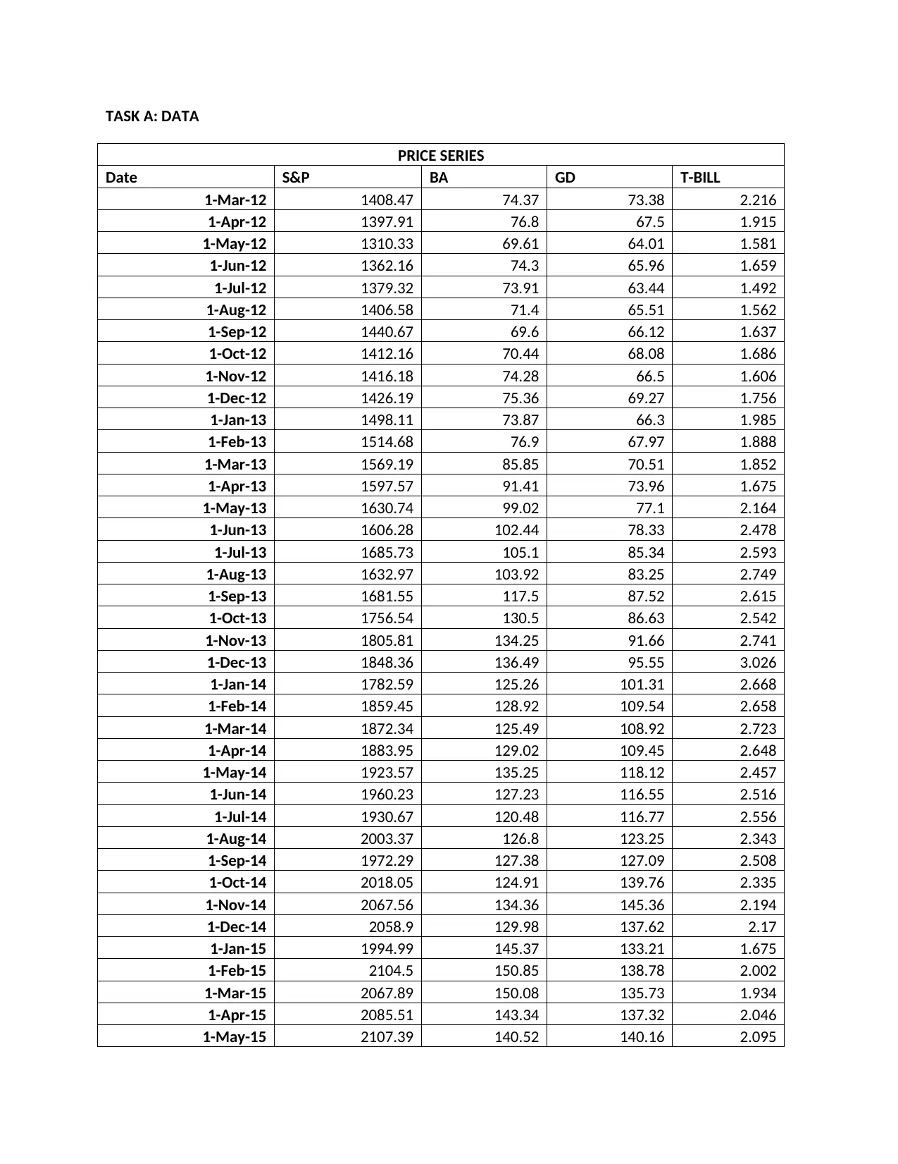
TASK A: DATA
PRICE SERIES
Date S&P BA GD T-BILL
1-Mar-12 1408.47 74.37 73.38 2.216
1-Apr-12 1397.91 76.8 67.5 1.915
1-May-12 1310.33 69.61 64.01 1.581
1-Jun-12 1362.16 74.3 65.96 1.659
1-Jul-12 1379.32 73.91 63.44 1.492
1-Aug-12 1406.58 71.4 65.51 1.562
1-Sep-12 1440.67 69.6 66.12 1.637
1-Oct-12 1412.16 70.44 68.08 1.686
1-Nov-12 1416.18 74.28 66.5 1.606
1-Dec-12 1426.19 75.36 69.27 1.756
1-Jan-13 1498.11 73.87 66.3 1.985
1-Feb-13 1514.68 76.9 67.97 1.888
1-Mar-13 1569.19 85.85 70.51 1.852
1-Apr-13 1597.57 91.41 73.96 1.675
1-May-13 1630.74 99.02 77.1 2.164
1-Jun-13 1606.28 102.44 78.33 2.478
1-Jul-13 1685.73 105.1 85.34 2.593
1-Aug-13 1632.97 103.92 83.25 2.749
1-Sep-13 1681.55 117.5 87.52 2.615
1-Oct-13 1756.54 130.5 86.63 2.542
1-Nov-13 1805.81 134.25 91.66 2.741
1-Dec-13 1848.36 136.49 95.55 3.026
1-Jan-14 1782.59 125.26 101.31 2.668
1-Feb-14 1859.45 128.92 109.54 2.658
1-Mar-14 1872.34 125.49 108.92 2.723
1-Apr-14 1883.95 129.02 109.45 2.648
1-May-14 1923.57 135.25 118.12 2.457
1-Jun-14 1960.23 127.23 116.55 2.516
1-Jul-14 1930.67 120.48 116.77 2.556
1-Aug-14 2003.37 126.8 123.25 2.343
1-Sep-14 1972.29 127.38 127.09 2.508
1-Oct-14 2018.05 124.91 139.76 2.335
1-Nov-14 2067.56 134.36 145.36 2.194
1-Dec-14 2058.9 129.98 137.62 2.17
1-Jan-15 1994.99 145.37 133.21 1.675
1-Feb-15 2104.5 150.85 138.78 2.002
1-Mar-15 2067.89 150.08 135.73 1.934
1-Apr-15 2085.51 143.34 137.32 2.046
1-May-15 2107.39 140.52 140.16 2.095
Secure Best Marks with AI Grader
Need help grading? Try our AI Grader for instant feedback on your assignments.
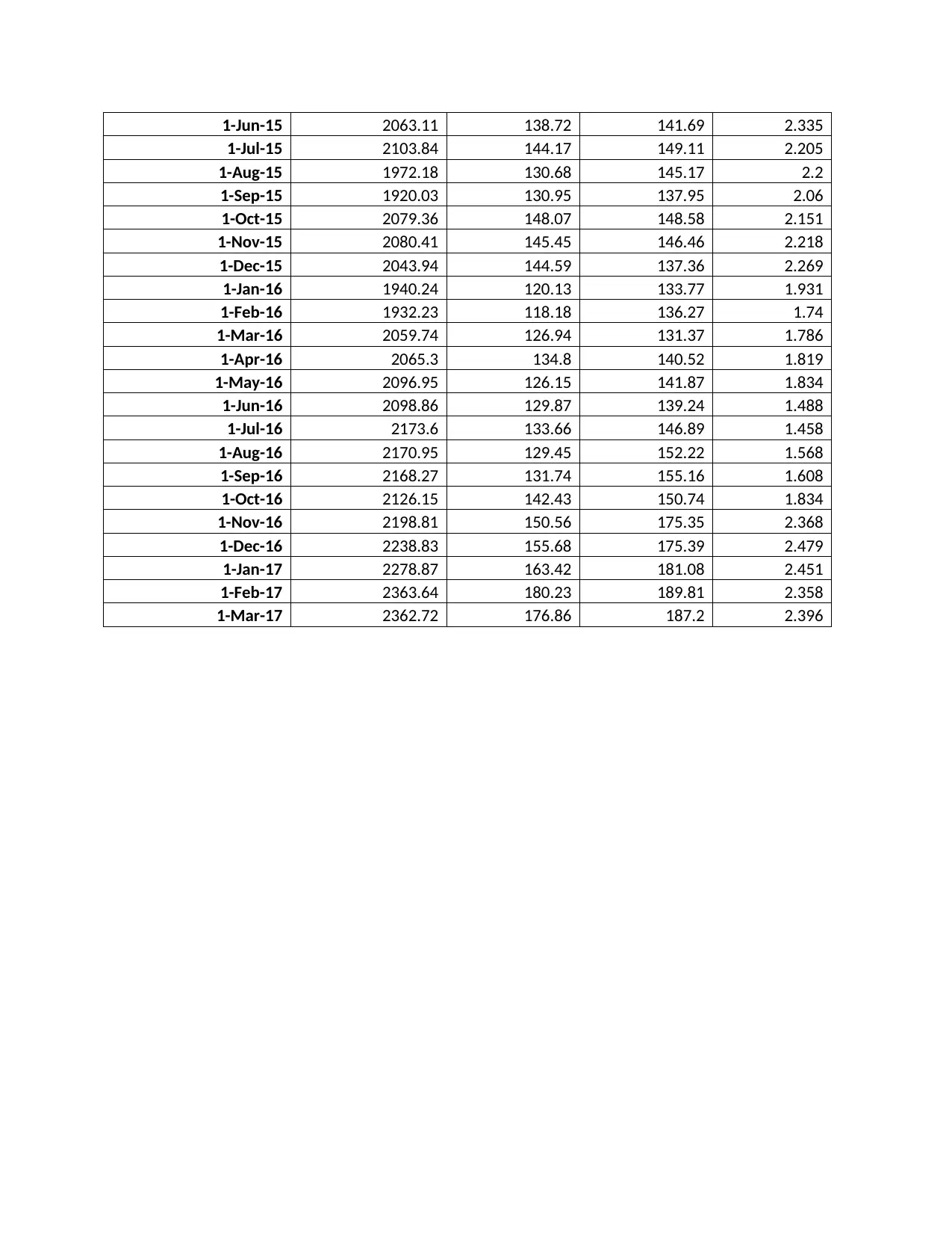
1-Jun-15 2063.11 138.72 141.69 2.335
1-Jul-15 2103.84 144.17 149.11 2.205
1-Aug-15 1972.18 130.68 145.17 2.2
1-Sep-15 1920.03 130.95 137.95 2.06
1-Oct-15 2079.36 148.07 148.58 2.151
1-Nov-15 2080.41 145.45 146.46 2.218
1-Dec-15 2043.94 144.59 137.36 2.269
1-Jan-16 1940.24 120.13 133.77 1.931
1-Feb-16 1932.23 118.18 136.27 1.74
1-Mar-16 2059.74 126.94 131.37 1.786
1-Apr-16 2065.3 134.8 140.52 1.819
1-May-16 2096.95 126.15 141.87 1.834
1-Jun-16 2098.86 129.87 139.24 1.488
1-Jul-16 2173.6 133.66 146.89 1.458
1-Aug-16 2170.95 129.45 152.22 1.568
1-Sep-16 2168.27 131.74 155.16 1.608
1-Oct-16 2126.15 142.43 150.74 1.834
1-Nov-16 2198.81 150.56 175.35 2.368
1-Dec-16 2238.83 155.68 175.39 2.479
1-Jan-17 2278.87 163.42 181.08 2.451
1-Feb-17 2363.64 180.23 189.81 2.358
1-Mar-17 2362.72 176.86 187.2 2.396
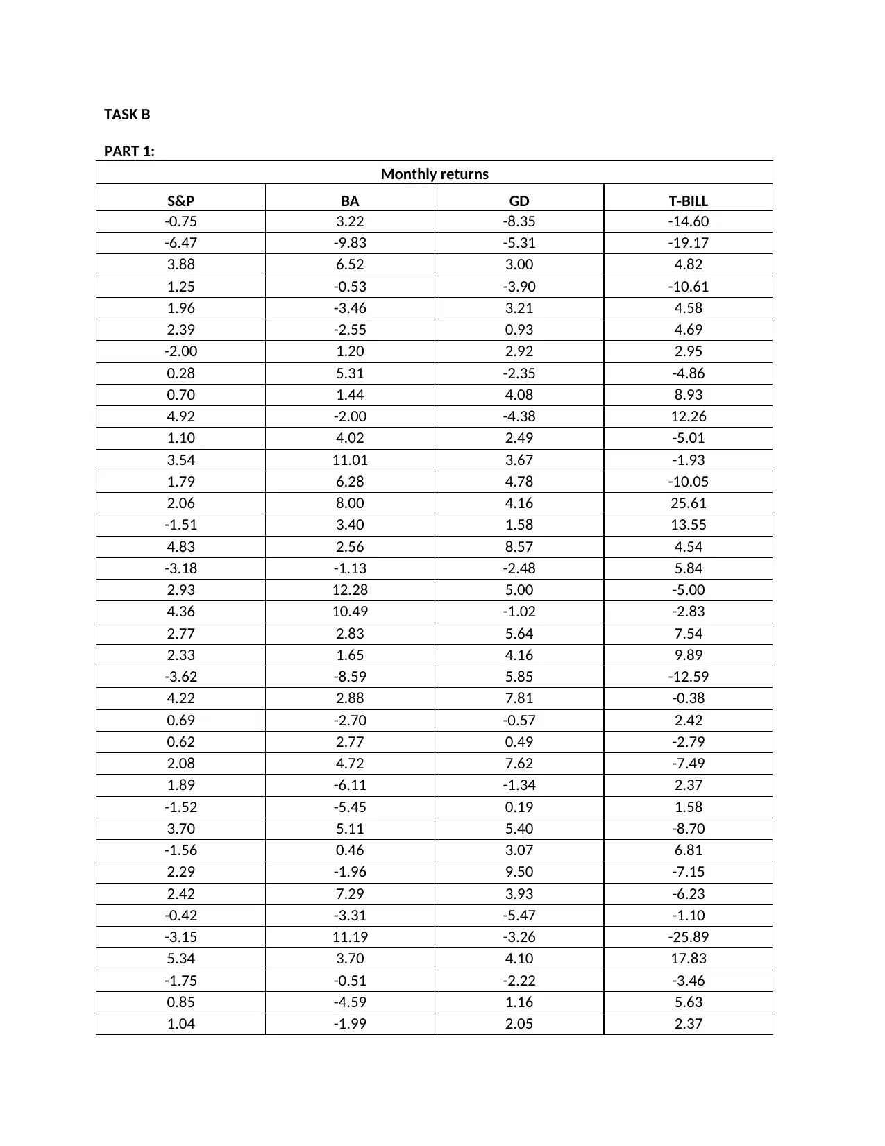
TASK B
PART 1:
Monthly returns
S&P BA GD T-BILL
-0.75 3.22 -8.35 -14.60
-6.47 -9.83 -5.31 -19.17
3.88 6.52 3.00 4.82
1.25 -0.53 -3.90 -10.61
1.96 -3.46 3.21 4.58
2.39 -2.55 0.93 4.69
-2.00 1.20 2.92 2.95
0.28 5.31 -2.35 -4.86
0.70 1.44 4.08 8.93
4.92 -2.00 -4.38 12.26
1.10 4.02 2.49 -5.01
3.54 11.01 3.67 -1.93
1.79 6.28 4.78 -10.05
2.06 8.00 4.16 25.61
-1.51 3.40 1.58 13.55
4.83 2.56 8.57 4.54
-3.18 -1.13 -2.48 5.84
2.93 12.28 5.00 -5.00
4.36 10.49 -1.02 -2.83
2.77 2.83 5.64 7.54
2.33 1.65 4.16 9.89
-3.62 -8.59 5.85 -12.59
4.22 2.88 7.81 -0.38
0.69 -2.70 -0.57 2.42
0.62 2.77 0.49 -2.79
2.08 4.72 7.62 -7.49
1.89 -6.11 -1.34 2.37
-1.52 -5.45 0.19 1.58
3.70 5.11 5.40 -8.70
-1.56 0.46 3.07 6.81
2.29 -1.96 9.50 -7.15
2.42 7.29 3.93 -6.23
-0.42 -3.31 -5.47 -1.10
-3.15 11.19 -3.26 -25.89
5.34 3.70 4.10 17.83
-1.75 -0.51 -2.22 -3.46
0.85 -4.59 1.16 5.63
1.04 -1.99 2.05 2.37
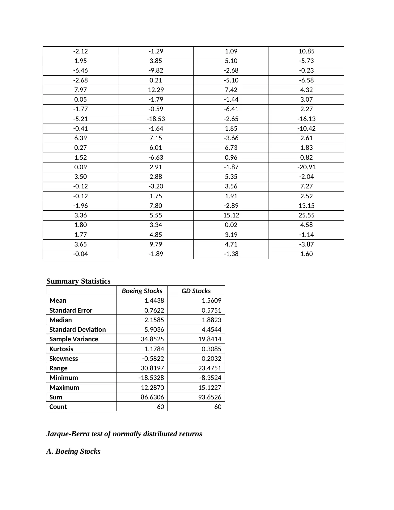
-2.12 -1.29 1.09 10.85
1.95 3.85 5.10 -5.73
-6.46 -9.82 -2.68 -0.23
-2.68 0.21 -5.10 -6.58
7.97 12.29 7.42 4.32
0.05 -1.79 -1.44 3.07
-1.77 -0.59 -6.41 2.27
-5.21 -18.53 -2.65 -16.13
-0.41 -1.64 1.85 -10.42
6.39 7.15 -3.66 2.61
0.27 6.01 6.73 1.83
1.52 -6.63 0.96 0.82
0.09 2.91 -1.87 -20.91
3.50 2.88 5.35 -2.04
-0.12 -3.20 3.56 7.27
-0.12 1.75 1.91 2.52
-1.96 7.80 -2.89 13.15
3.36 5.55 15.12 25.55
1.80 3.34 0.02 4.58
1.77 4.85 3.19 -1.14
3.65 9.79 4.71 -3.87
-0.04 -1.89 -1.38 1.60
Summary Statistics
Boeing Stocks GD Stocks
Mean 1.4438 1.5609
Standard Error 0.7622 0.5751
Median 2.1585 1.8823
Standard Deviation 5.9036 4.4544
Sample Variance 34.8525 19.8414
Kurtosis 1.1784 0.3085
Skewness -0.5822 0.2032
Range 30.8197 23.4751
Minimum -18.5328 -8.3524
Maximum 12.2870 15.1227
Sum 86.6306 93.6526
Count 60 60
Jarque-Berra test of normally distributed returns
A. Boeing Stocks
Secure Best Marks with AI Grader
Need help grading? Try our AI Grader for instant feedback on your assignments.
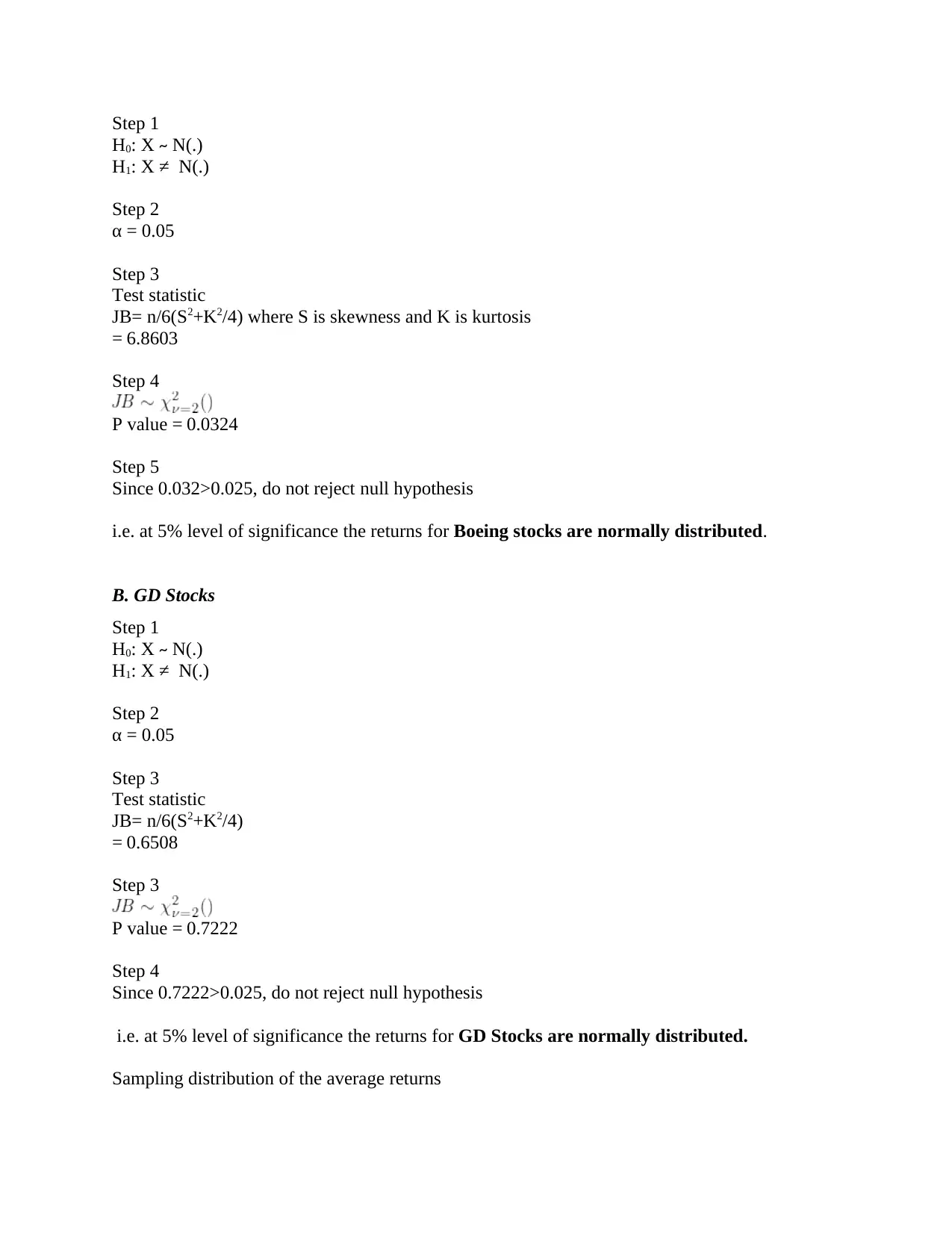
Step 1
H0: X ~ N(.)
H1: X ≠ N(.)
Step 2
α = 0.05
Step 3
Test statistic
JB= n/6(S2+K2/4) where S is skewness and K is kurtosis
= 6.8603
Step 4
P value = 0.0324
Step 5
Since 0.032>0.025, do not reject null hypothesis
i.e. at 5% level of significance the returns for Boeing stocks are normally distributed.
B. GD Stocks
Step 1
H0: X ~ N(.)
H1: X ≠ N(.)
Step 2
α = 0.05
Step 3
Test statistic
JB= n/6(S2+K2/4)
= 0.6508
Step 3
P value = 0.7222
Step 4
Since 0.7222>0.025, do not reject null hypothesis
i.e. at 5% level of significance the returns for GD Stocks are normally distributed.
Sampling distribution of the average returns
H0: X ~ N(.)
H1: X ≠ N(.)
Step 2
α = 0.05
Step 3
Test statistic
JB= n/6(S2+K2/4) where S is skewness and K is kurtosis
= 6.8603
Step 4
P value = 0.0324
Step 5
Since 0.032>0.025, do not reject null hypothesis
i.e. at 5% level of significance the returns for Boeing stocks are normally distributed.
B. GD Stocks
Step 1
H0: X ~ N(.)
H1: X ≠ N(.)
Step 2
α = 0.05
Step 3
Test statistic
JB= n/6(S2+K2/4)
= 0.6508
Step 3
P value = 0.7222
Step 4
Since 0.7222>0.025, do not reject null hypothesis
i.e. at 5% level of significance the returns for GD Stocks are normally distributed.
Sampling distribution of the average returns
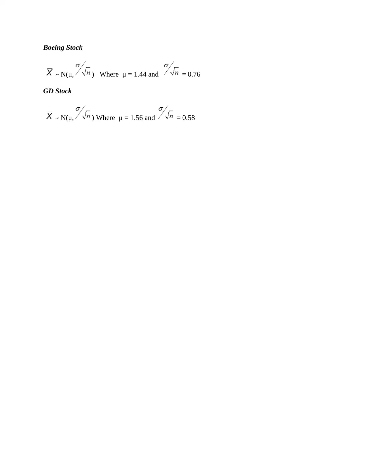
Boeing Stock
~ N(μ, ) Where μ = 1.44 and = 0.76
GD Stock
~ N(μ, ) Where μ = 1.56 and = 0.58
~ N(μ, ) Where μ = 1.44 and = 0.76
GD Stock
~ N(μ, ) Where μ = 1.56 and = 0.58
PART 2:
Single population mean
Test statistic: t statistic
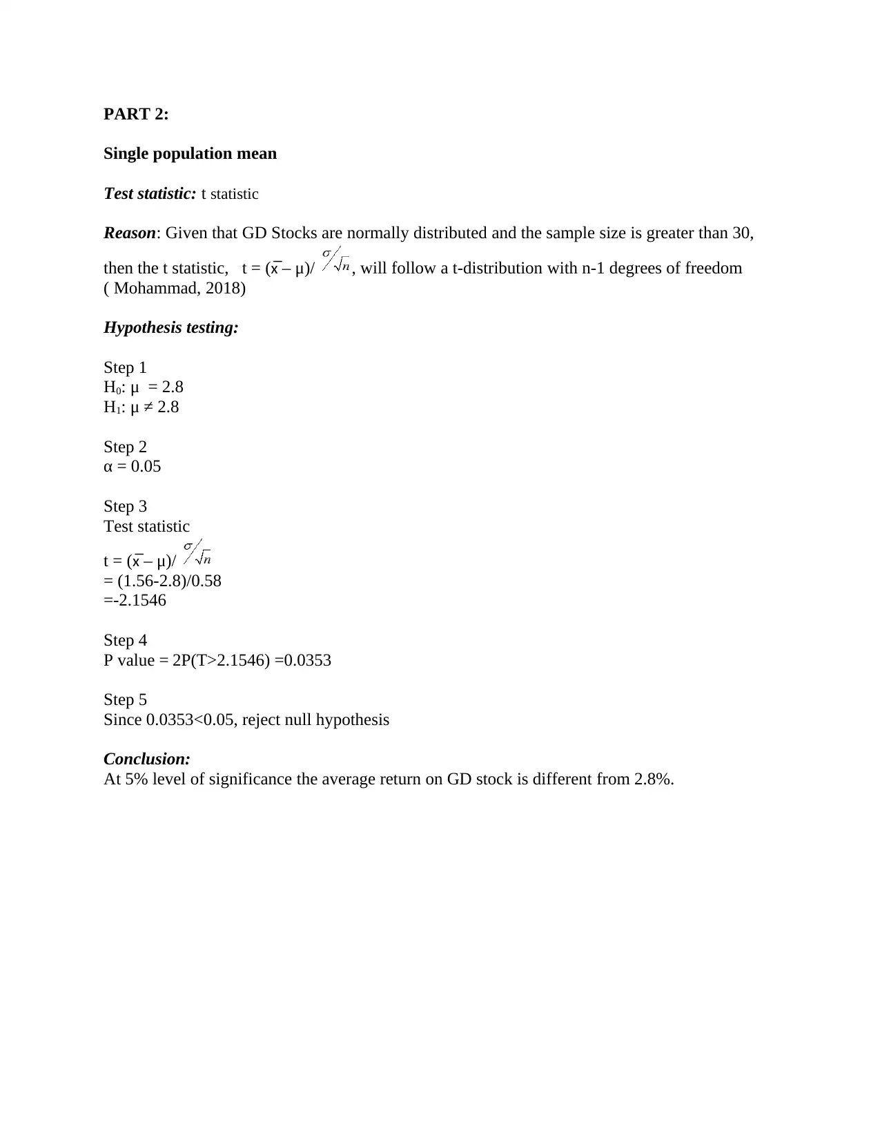
Reason: Given that GD Stocks are normally distributed and the sample size is greater than 30,
then the t statistic, t = (x̅ – μ)/ , will follow a t-distribution with n-1 degrees of freedom
( Mohammad, 2018)
Hypothesis testing:
Step 1
H0: μ = 2.8
H1: μ ≠ 2.8
Step 2
α = 0.05
Step 3
Test statistic
t = (x̅ – μ)/
= (1.56-2.8)/0.58
=-2.1546
Step 4
P value = 2P(T>2.1546) =0.0353
Step 5
Since 0.0353<0.05, reject null hypothesis
Conclusion:
At 5% level of significance the average return on GD stock is different from 2.8%.
Paraphrase This Document
Need a fresh take? Get an instant paraphrase of this document with our AI Paraphraser
PART 3: Testing of Homoscedasticity
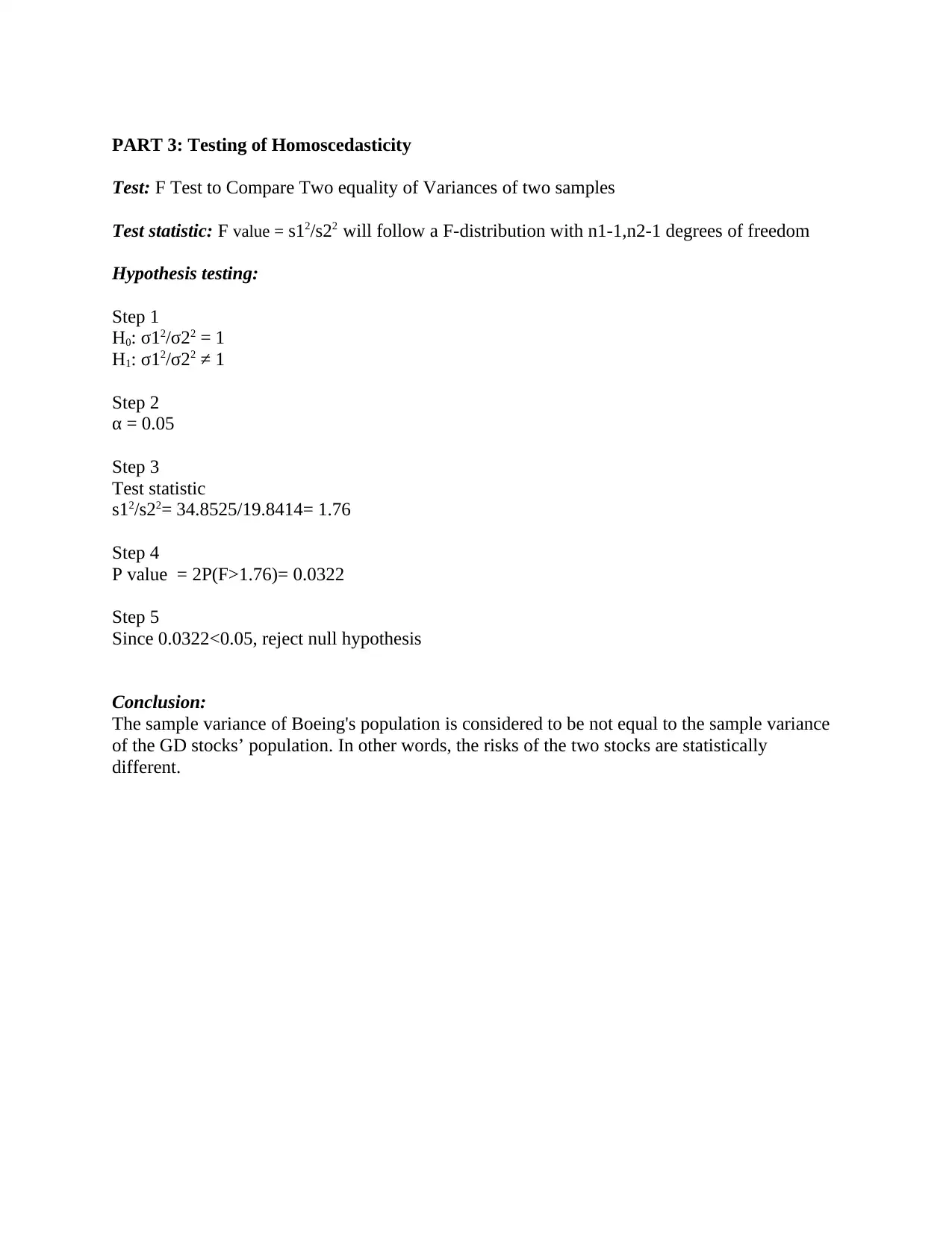
Test: F Test to Compare Two equality of Variances of two samples
Test statistic: F value = s12/s22 will follow a F-distribution with n1-1,n2-1 degrees of freedom
Hypothesis testing:
Step 1
H0: σ12/σ22 = 1
H1: σ12/σ22 ≠ 1
Step 2
α = 0.05
Step 3
Test statistic
s12/s22= 34.8525/19.8414= 1.76
Step 4
P value = 2P(F>1.76)= 0.0322
Step 5
Since 0.0322<0.05, reject null hypothesis
Conclusion:
The sample variance of Boeing's population is considered to be not equal to the sample variance
of the GD stocks’ population. In other words, the risks of the two stocks are statistically
different.
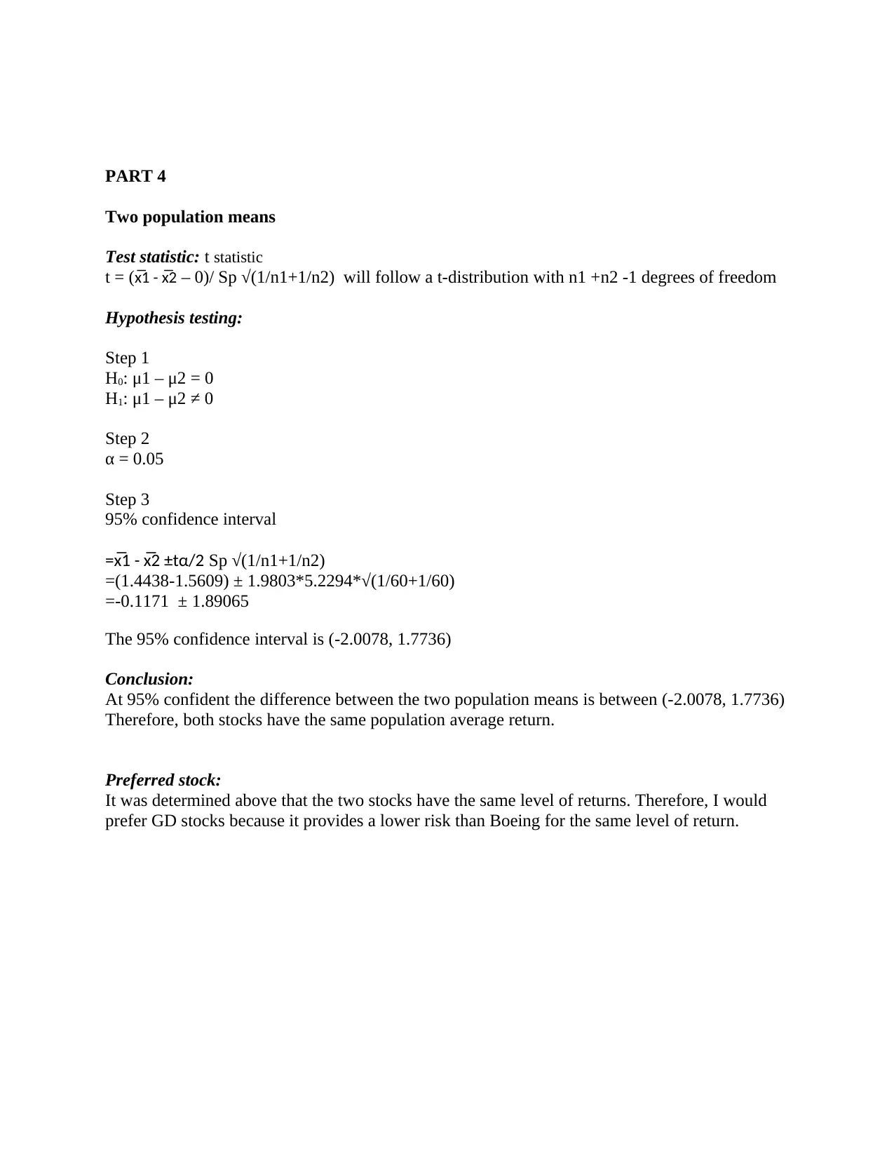
PART 4
Two population means
Test statistic: t statistic
t = (x̅1 - x̅2 – 0)/ Sp √(1/n1+1/n2) will follow a t-distribution with n1 +n2 -1 degrees of freedom
Hypothesis testing:
Step 1
H0: μ1 – μ2 = 0
H1: μ1 – μ2 ≠ 0
Step 2
α = 0.05
Step 3
95% confidence interval
=x̅1 - x̅2 ±tα/2 Sp √(1/n1+1/n2)
=(1.4438-1.5609) ± 1.9803*5.2294*√(1/60+1/60)
=-0.1171 ± 1.89065
The 95% confidence interval is (-2.0078, 1.7736)
Conclusion:
At 95% confident the difference between the two population means is between (-2.0078, 1.7736)
Therefore, both stocks have the same population average return.
Preferred stock:
It was determined above that the two stocks have the same level of returns. Therefore, I would
prefer GD stocks because it provides a lower risk than Boeing for the same level of return.
TASK C
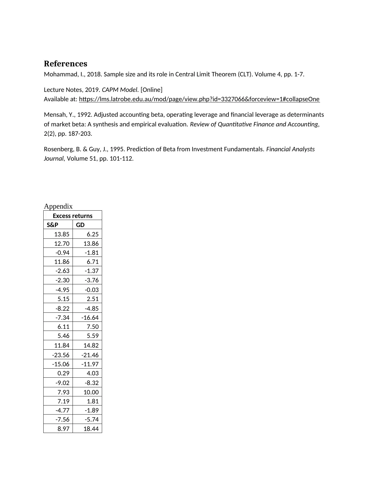
a) CAPM Beta
Re= Rf + Beta*(Rm –Rf), where Rf is the risk free rate and Rm is the return on the market
ßi = cov (Ri,Rm)/var(Rm) (Mensah, 1992)
To estimate the beta of a particular stock,
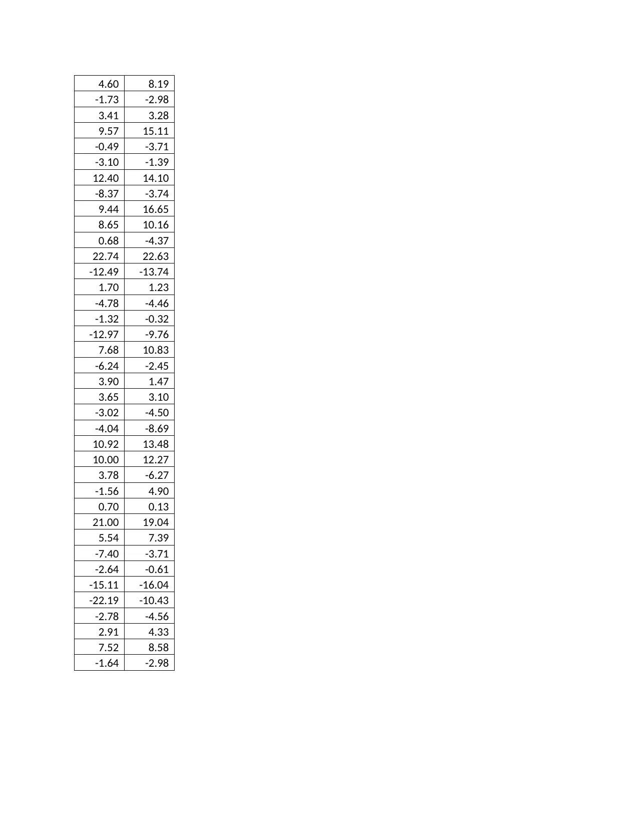
-Regress (excess) returns on the stock against (excess) returns on the “market portfolio (see
appendix) (Lecture Notes, 2019)
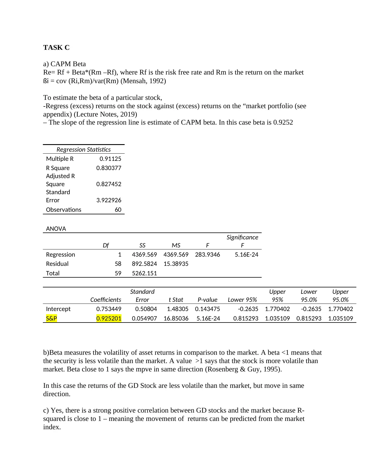
– The slope of the regression line is estimate of CAPM beta. In this case beta is 0.9252
Regression Statistics
Multiple R 0.91125
R Square 0.830377
Adjusted R
Square 0.827452
Standard
Error 3.922926
Observations 60
ANOVA
Df SS MS F
Significance
F
Regression 1 4369.569 4369.569 283.9346 5.16E-24
Residual 58 892.5824 15.38935
Total 59 5262.151
Coefficients
Standard
Error t Stat P-value Lower 95%
Upper
95%
Lower
95.0%
Upper
95.0%
Intercept 0.753449 0.50804 1.48305 0.143475 -0.2635 1.770402 -0.2635 1.770402
S&P 0.925201 0.054907 16.85036 5.16E-24 0.815293 1.035109 0.815293 1.035109
b)Beta measures the volatility of asset returns in comparison to the market. A beta <1 means that
the security is less volatile than the market. A value >1 says that the stock is more volatile than
market. Beta close to 1 says the mpve in same direction (Rosenberg & Guy, 1995).
In this case the returns of the GD Stock are less volatile than the market, but move in same
direction.
c) Yes, there is a strong positive correlation between GD stocks and the market because R-
squared is close to 1 – meaning the movement of returns can be predicted from the market
index.
Secure Best Marks with AI Grader
Need help grading? Try our AI Grader for instant feedback on your assignments.
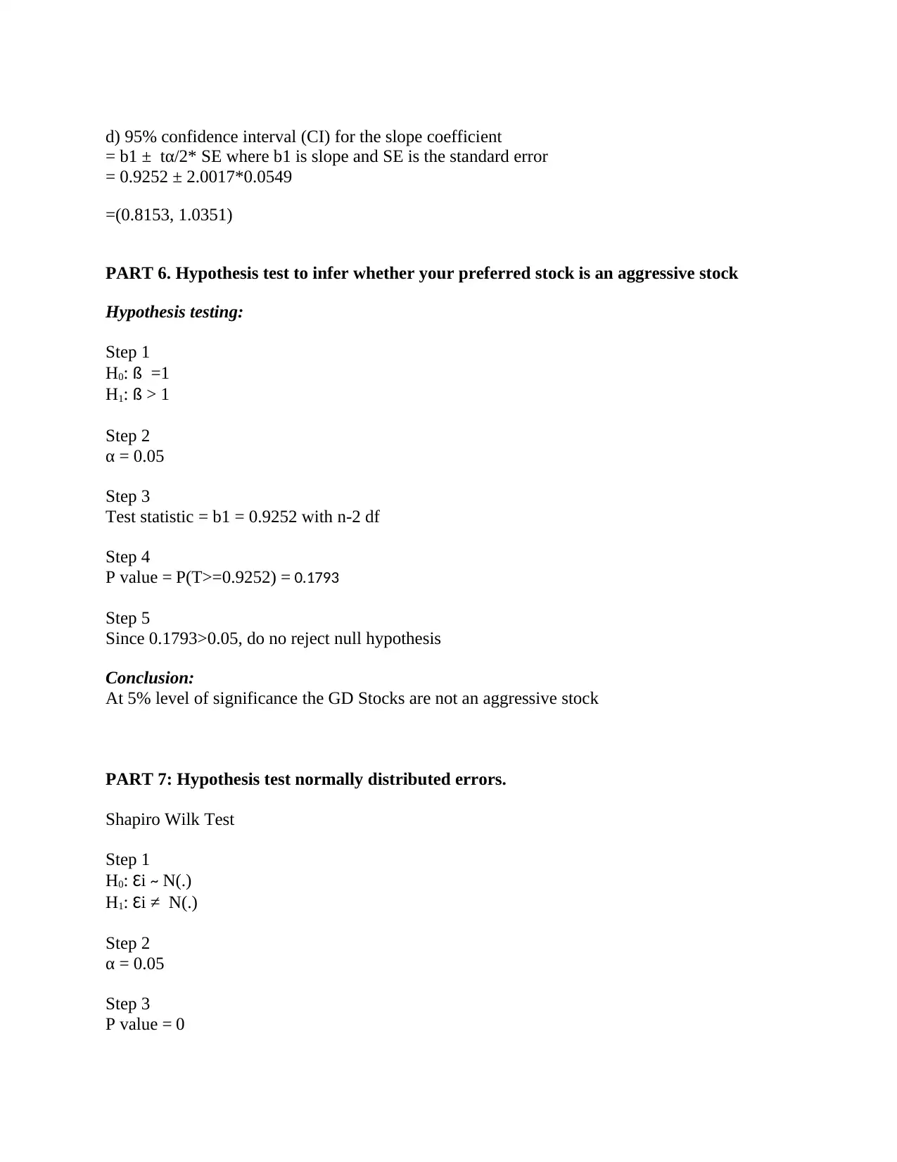
d) 95% confidence interval (CI) for the slope coefficient
= b1 ± tα/2* SE where b1 is slope and SE is the standard error
= 0.9252 ± 2.0017*0.0549
=(0.8153, 1.0351)
PART 6. Hypothesis test to infer whether your preferred stock is an aggressive stock
Hypothesis testing:
Step 1
H0: ß =1
H1: ß > 1
Step 2
α = 0.05
Step 3
Test statistic = b1 = 0.9252 with n-2 df
Step 4
P value = P(T>=0.9252) = 0.1793
Step 5
Since 0.1793>0.05, do no reject null hypothesis
Conclusion:
At 5% level of significance the GD Stocks are not an aggressive stock
PART 7: Hypothesis test normally distributed errors.
Shapiro Wilk Test
Step 1
H0: Ɛi ~ N(.)
H1: Ɛi ≠ N(.)
Step 2
α = 0.05
Step 3
P value = 0
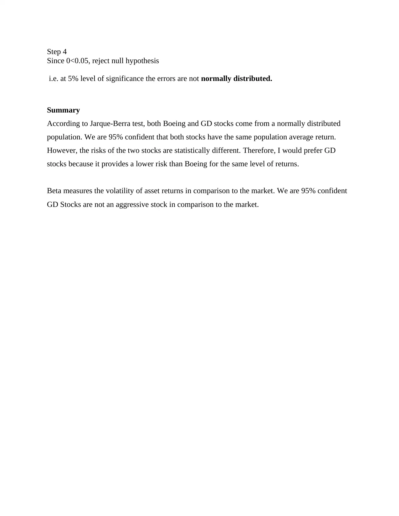
Step 4
Since 0<0.05, reject null hypothesis
i.e. at 5% level of significance the errors are not normally distributed.
Summary
According to Jarque-Berra test, both Boeing and GD stocks come from a normally distributed
population. We are 95% confident that both stocks have the same population average return.
However, the risks of the two stocks are statistically different. Therefore, I would prefer GD
stocks because it provides a lower risk than Boeing for the same level of returns.
Beta measures the volatility of asset returns in comparison to the market. We are 95% confident
GD Stocks are not an aggressive stock in comparison to the market.
References
Mohammad, I., 2018. Sample size and its role in Central Limit Theorem (CLT). Volume 4, pp. 1-7.
Lecture Notes, 2019. CAPM Model. [Online]
Available at: https://lms.latrobe.edu.au/mod/page/view.php?id=3327066&forceview=1#collapseOne
Mensah, Y., 1992. Adjusted accounting beta, operating leverage and financial leverage as determinants
of market beta: A synthesis and empirical evaluation. Review of Quantitative Finance and Accounting,
2(2), pp. 187-203.
Rosenberg, B. & Guy, J., 1995. Prediction of Beta from Investment Fundamentals. Financial Analysts
Journal, Volume 51, pp. 101-112.
Appendix
Excess returns
S&P GD
13.85 6.25
12.70 13.86
-0.94 -1.81
11.86 6.71
-2.63 -1.37
-2.30 -3.76
-4.95 -0.03
5.15 2.51
-8.22 -4.85
-7.34 -16.64
6.11 7.50
5.46 5.59
11.84 14.82
-23.56 -21.46
-15.06 -11.97
0.29 4.03
-9.02 -8.32
7.93 10.00
7.19 1.81
-4.77 -1.89
-7.56 -5.74
8.97 18.44
Paraphrase This Document
Need a fresh take? Get an instant paraphrase of this document with our AI Paraphraser
4.60 8.19
-1.73 -2.98
3.41 3.28
9.57 15.11
-0.49 -3.71
-3.10 -1.39
12.40 14.10
-8.37 -3.74
9.44 16.65
8.65 10.16
0.68 -4.37
22.74 22.63
-12.49 -13.74
1.70 1.23
-4.78 -4.46
-1.32 -0.32
-12.97 -9.76
7.68 10.83
-6.24 -2.45
3.90 1.47
3.65 3.10
-3.02 -4.50
-4.04 -8.69
10.92 13.48
10.00 12.27
3.78 -6.27
-1.56 4.90
0.70 0.13
21.00 19.04
5.54 7.39
-7.40 -3.71
-2.64 -0.61
-15.11 -16.04
-22.19 -10.43
-2.78 -4.56
2.91 4.33
7.52 8.58
-1.64 -2.98
1 out of 14
Related Documents
Your All-in-One AI-Powered Toolkit for Academic Success.
+13062052269
info@desklib.com
Available 24*7 on WhatsApp / Email
![[object Object]](/_next/static/media/star-bottom.7253800d.svg)
Unlock your academic potential
© 2024 | Zucol Services PVT LTD | All rights reserved.


