Transport Economics - Desklib Online Library
Added on 2023-06-15
17 Pages2721 Words299 Views
Running Head: TRANSPORT ECONOMICS
Transport Economics
Name of the Student
Name of the University
Author note
Transport Economics
Name of the Student
Name of the University
Author note

1TRANSPORT ECONOMICS
Table of Contents
Task 1.........................................................................................................................................2
Task 2.........................................................................................................................................3
Bivariate regression................................................................................................................3
Residual plot...........................................................................................................................7
Task 3.........................................................................................................................................9
Model 1..................................................................................................................................9
Model 2................................................................................................................................11
Model 3....................................................................................................................................12
Task 4.......................................................................................................................................14
Forecast................................................................................................................................14
References................................................................................................................................16
2TRANSPORT ECONOMICS
Task 1
- 5,000,000 10,000,000 15,000,000 20,000,000 25,000,000
-
10,000,000
20,000,000
30,000,000
40,000,000
50,000,000
60,000,000
70,000,000
80,000,000
-
10,000,000
20,000,000
30,000,000
40,000,000
50,000,000
60,000,000
70,000,000
80,000,000
f(x) = 922.330951872083 x + 2851837.16103047
R² = 0.977320752162377 f(x) = 5.87873434629525 x − 74877468.3237875
R² = 0.945320839513967
R² = 0R² = 0
Scatter Plot
International tourism, number of departures (X2)
Linear (International tourism, number of departures (X2))
International tourism, number of arrivals (X3)
Linear (International tourism, number of arrivals (X3))
Population (X4)
Linear (Population (X4))
GDP per capita (X1)
Linear (GDP per capita (X1))
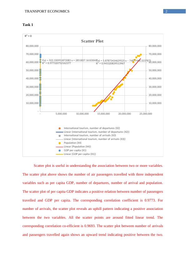
Scatter plot is useful in understanding the association between two or more variables.
The scatter plot above shows the number of air passengers travelled with three independent
variables such as per capita GDP, number of departures, number of arrival and population.
The scatter plot of per capita GDP indicates a positive relation between number of passengers
travelled and GDP per capita. The corresponding correlation coefficient is 0.9773. For
number of arrivals, the scatter plot reveals an uphill pattern indicating a positive association
between the two variables. All the scatter points are around fitted linear trend. The
corresponding correlation co-efficient is 0.9693. The scatter plot between number of arrivals
and passengers travelled again shows an upward trend indicating positive between the two.
Task 1
- 5,000,000 10,000,000 15,000,000 20,000,000 25,000,000
-
10,000,000
20,000,000
30,000,000
40,000,000
50,000,000
60,000,000
70,000,000
80,000,000
-
10,000,000
20,000,000
30,000,000
40,000,000
50,000,000
60,000,000
70,000,000
80,000,000
f(x) = 922.330951872083 x + 2851837.16103047
R² = 0.977320752162377 f(x) = 5.87873434629525 x − 74877468.3237875
R² = 0.945320839513967
R² = 0R² = 0
Scatter Plot
International tourism, number of departures (X2)
Linear (International tourism, number of departures (X2))
International tourism, number of arrivals (X3)
Linear (International tourism, number of arrivals (X3))
Population (X4)
Linear (Population (X4))
GDP per capita (X1)
Linear (GDP per capita (X1))
Scatter plot is useful in understanding the association between two or more variables.
The scatter plot above shows the number of air passengers travelled with three independent
variables such as per capita GDP, number of departures, number of arrival and population.
The scatter plot of per capita GDP indicates a positive relation between number of passengers
travelled and GDP per capita. The corresponding correlation coefficient is 0.9773. For
number of arrivals, the scatter plot reveals an uphill pattern indicating a positive association
between the two variables. All the scatter points are around fitted linear trend. The
corresponding correlation co-efficient is 0.9693. The scatter plot between number of arrivals
and passengers travelled again shows an upward trend indicating positive between the two.
3TRANSPORT ECONOMICS
Population also has a positive relation with passengers travelled. Therefore, all the variables
have a linear relationship with the dependent variables. Scatter plot however shows only
degree of association (Fox, 2015). It does not indicate any cause and effect relation. For the
later, a regression needs to be done.
Task 2
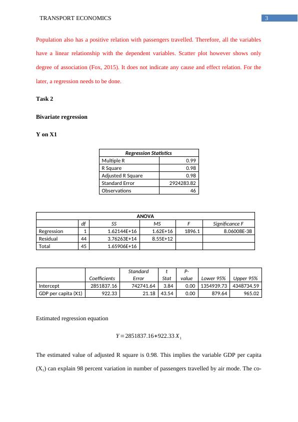
Bivariate regression
Y on X1
Regression Statistics
Multiple R 0.99
R Square 0.98
Adjusted R Square 0.98
Standard Error 2924283.82
Observations 46
ANOVA
df SS MS F Significance F
Regression 1 1.62144E+16 1.62E+16 1896.1 8.06008E-38
Residual 44 3.76263E+14 8.55E+12
Total 45 1.65906E+16
Coefficients
Standard
Error
t
Stat
P-
value Lower 95% Upper 95%
Intercept 2851837.16 742741.64 3.84 0.00 1354939.73 4348734.59
GDP per capita (X1) 922.33 21.18 43.54 0.00 879.64 965.02
Estimated regression equation
Y =2851837.16+922.33 X1
The estimated value of adjusted R square is 0.98. This implies the variable GDP per capita
(X1) can explain 98 percent variation in number of passengers travelled by air mode. The co-
Population also has a positive relation with passengers travelled. Therefore, all the variables
have a linear relationship with the dependent variables. Scatter plot however shows only
degree of association (Fox, 2015). It does not indicate any cause and effect relation. For the
later, a regression needs to be done.
Task 2
Bivariate regression
Y on X1
Regression Statistics
Multiple R 0.99
R Square 0.98
Adjusted R Square 0.98
Standard Error 2924283.82
Observations 46
ANOVA
df SS MS F Significance F
Regression 1 1.62144E+16 1.62E+16 1896.1 8.06008E-38
Residual 44 3.76263E+14 8.55E+12
Total 45 1.65906E+16
Coefficients
Standard
Error
t
Stat
P-
value Lower 95% Upper 95%
Intercept 2851837.16 742741.64 3.84 0.00 1354939.73 4348734.59
GDP per capita (X1) 922.33 21.18 43.54 0.00 879.64 965.02
Estimated regression equation
Y =2851837.16+922.33 X1
The estimated value of adjusted R square is 0.98. This implies the variable GDP per capita
(X1) can explain 98 percent variation in number of passengers travelled by air mode. The co-
End of preview
Want to access all the pages? Upload your documents or become a member.
Related Documents
Predictive Demand Analysislg...
|13
|1536
|157