Optimizing Transportation Cost and Recycled Garbage Amount
VerifiedAdded on 2023/06/11
|15
|2189
|274
AI Summary
This article discusses the optimization of transportation cost and recycled garbage amount using a multiple-objective linear programming (MOLP) model. The MOLP model is implemented in an Excel spreadsheet. The article also includes a GP model to optimize both objectives simultaneously. Additionally, the article covers finding the priority of factors for selecting a van and selecting the best location based on multiple criteria.
Contribute Materials
Your contribution can guide someone’s learning journey. Share your
documents today.
Solution
Q1)
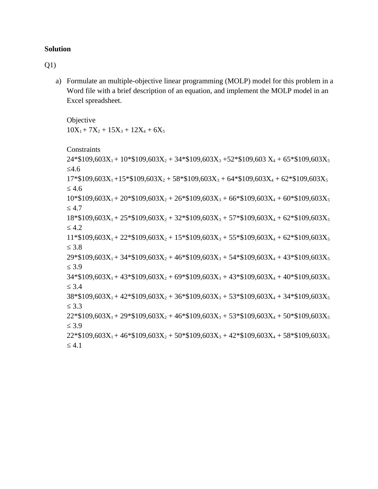
a) Formulate an multiple-objective linear programming (MOLP) model for this problem in a
Word file with a brief description of an equation, and implement the MOLP model in an
Excel spreadsheet.
Objective
10X1 + 7X2 + 15X3 + 12X4 + 6X5
Constraints
24*$109,603X1 + 10*$109,603X2 + 34*$109,603X3 +52*$109,603 X4 + 65*$109,603X5
≤4.6
17*$109,603X1 +15*$109,603X2 + 58*$109,603X3 + 64*$109,603X4 + 62*$109,603X5
≤ 4.6
10*$109,603X1 + 20*$109,603X2 + 26*$109,603X3 + 66*$109,603X4 + 60*$109,603X5
≤ 4.7
18*$109,603X1 + 25*$109,603X2 + 32*$109,603X3 + 57*$109,603X4 + 62*$109,603X5
≤ 4.2
11*$109,603X1 + 22*$109,603X2 + 15*$109,603X3 + 55*$109,603X4 + 62*$109,603X5
≤ 3.8
29*$109,603X1 + 34*$109,603X2 + 46*$109,603X3 + 54*$109,603X4 + 43*$109,603X5
≤ 3.9
34*$109,603X1 + 43*$109,603X2 + 69*$109,603X3 + 43*$109,603X4 + 40*$109,603X5
≤ 3.4
38*$109,603X1 + 42*$109,603X2 + 36*$109,603X3 + 53*$109,603X4 + 34*$109,603X5
≤ 3.3
22*$109,603X1 + 29*$109,603X2 + 46*$109,603X3 + 53*$109,603X4 + 50*$109,603X5
≤ 3.9
22*$109,603X1 + 46*$109,603X2 + 50*$109,603X3 + 42*$109,603X4 + 58*$109,603X5
≤ 4.1
Q1)
a) Formulate an multiple-objective linear programming (MOLP) model for this problem in a
Word file with a brief description of an equation, and implement the MOLP model in an
Excel spreadsheet.
Objective
10X1 + 7X2 + 15X3 + 12X4 + 6X5
Constraints
24*$109,603X1 + 10*$109,603X2 + 34*$109,603X3 +52*$109,603 X4 + 65*$109,603X5
≤4.6
17*$109,603X1 +15*$109,603X2 + 58*$109,603X3 + 64*$109,603X4 + 62*$109,603X5
≤ 4.6
10*$109,603X1 + 20*$109,603X2 + 26*$109,603X3 + 66*$109,603X4 + 60*$109,603X5
≤ 4.7
18*$109,603X1 + 25*$109,603X2 + 32*$109,603X3 + 57*$109,603X4 + 62*$109,603X5
≤ 4.2
11*$109,603X1 + 22*$109,603X2 + 15*$109,603X3 + 55*$109,603X4 + 62*$109,603X5
≤ 3.8
29*$109,603X1 + 34*$109,603X2 + 46*$109,603X3 + 54*$109,603X4 + 43*$109,603X5
≤ 3.9
34*$109,603X1 + 43*$109,603X2 + 69*$109,603X3 + 43*$109,603X4 + 40*$109,603X5
≤ 3.4
38*$109,603X1 + 42*$109,603X2 + 36*$109,603X3 + 53*$109,603X4 + 34*$109,603X5
≤ 3.3
22*$109,603X1 + 29*$109,603X2 + 46*$109,603X3 + 53*$109,603X4 + 50*$109,603X5
≤ 3.9
22*$109,603X1 + 46*$109,603X2 + 50*$109,603X3 + 42*$109,603X4 + 58*$109,603X5
≤ 4.1
Secure Best Marks with AI Grader
Need help grading? Try our AI Grader for instant feedback on your assignments.
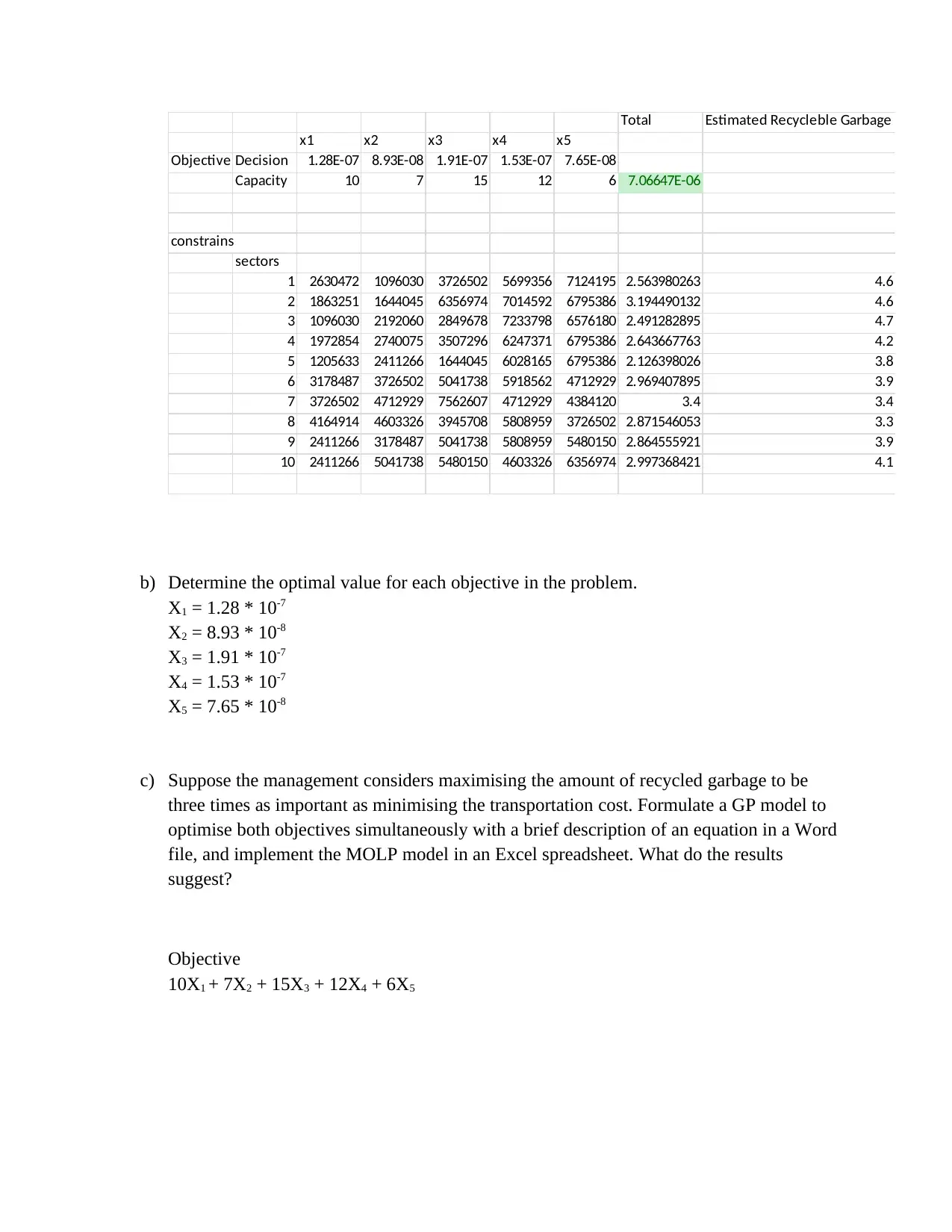
Total Estimated Recycleble Garbage
x1 x2 x3 x4 x5
Objective Decision 1.28E-07 8.93E-08 1.91E-07 1.53E-07 7.65E-08
Capacity 10 7 15 12 6 7.06647E-06
constrains
sectors
1 2630472 1096030 3726502 5699356 7124195 2.563980263 4.6
2 1863251 1644045 6356974 7014592 6795386 3.194490132 4.6
3 1096030 2192060 2849678 7233798 6576180 2.491282895 4.7
4 1972854 2740075 3507296 6247371 6795386 2.643667763 4.2
5 1205633 2411266 1644045 6028165 6795386 2.126398026 3.8
6 3178487 3726502 5041738 5918562 4712929 2.969407895 3.9
7 3726502 4712929 7562607 4712929 4384120 3.4 3.4
8 4164914 4603326 3945708 5808959 3726502 2.871546053 3.3
9 2411266 3178487 5041738 5808959 5480150 2.864555921 3.9
10 2411266 5041738 5480150 4603326 6356974 2.997368421 4.1
b) Determine the optimal value for each objective in the problem.
X1 = 1.28 * 10-7
X2 = 8.93 * 10-8
X3 = 1.91 * 10-7
X4 = 1.53 * 10-7
X5 = 7.65 * 10-8
c) Suppose the management considers maximising the amount of recycled garbage to be
three times as important as minimising the transportation cost. Formulate a GP model to
optimise both objectives simultaneously with a brief description of an equation in a Word
file, and implement the MOLP model in an Excel spreadsheet. What do the results
suggest?
Objective
10X1 + 7X2 + 15X3 + 12X4 + 6X5
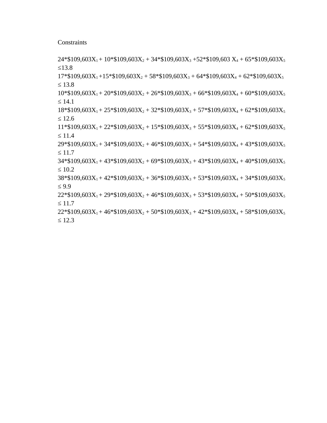
Constraints
24*$109,603X1 + 10*$109,603X2 + 34*$109,603X3 +52*$109,603 X4 + 65*$109,603X5
≤13.8
17*$109,603X1 +15*$109,603X2 + 58*$109,603X3 + 64*$109,603X4 + 62*$109,603X5
≤ 13.8
10*$109,603X1 + 20*$109,603X2 + 26*$109,603X3 + 66*$109,603X4 + 60*$109,603X5
≤ 14.1
18*$109,603X1 + 25*$109,603X2 + 32*$109,603X3 + 57*$109,603X4 + 62*$109,603X5
≤ 12.6
11*$109,603X1 + 22*$109,603X2 + 15*$109,603X3 + 55*$109,603X4 + 62*$109,603X5
≤ 11.4
29*$109,603X1 + 34*$109,603X2 + 46*$109,603X3 + 54*$109,603X4 + 43*$109,603X5
≤ 11.7
34*$109,603X1 + 43*$109,603X2 + 69*$109,603X3 + 43*$109,603X4 + 40*$109,603X5
≤ 10.2
38*$109,603X1 + 42*$109,603X2 + 36*$109,603X3 + 53*$109,603X4 + 34*$109,603X5
≤ 9.9
22*$109,603X1 + 29*$109,603X2 + 46*$109,603X3 + 53*$109,603X4 + 50*$109,603X5
≤ 11.7
22*$109,603X1 + 46*$109,603X2 + 50*$109,603X3 + 42*$109,603X4 + 58*$109,603X5
≤ 12.3
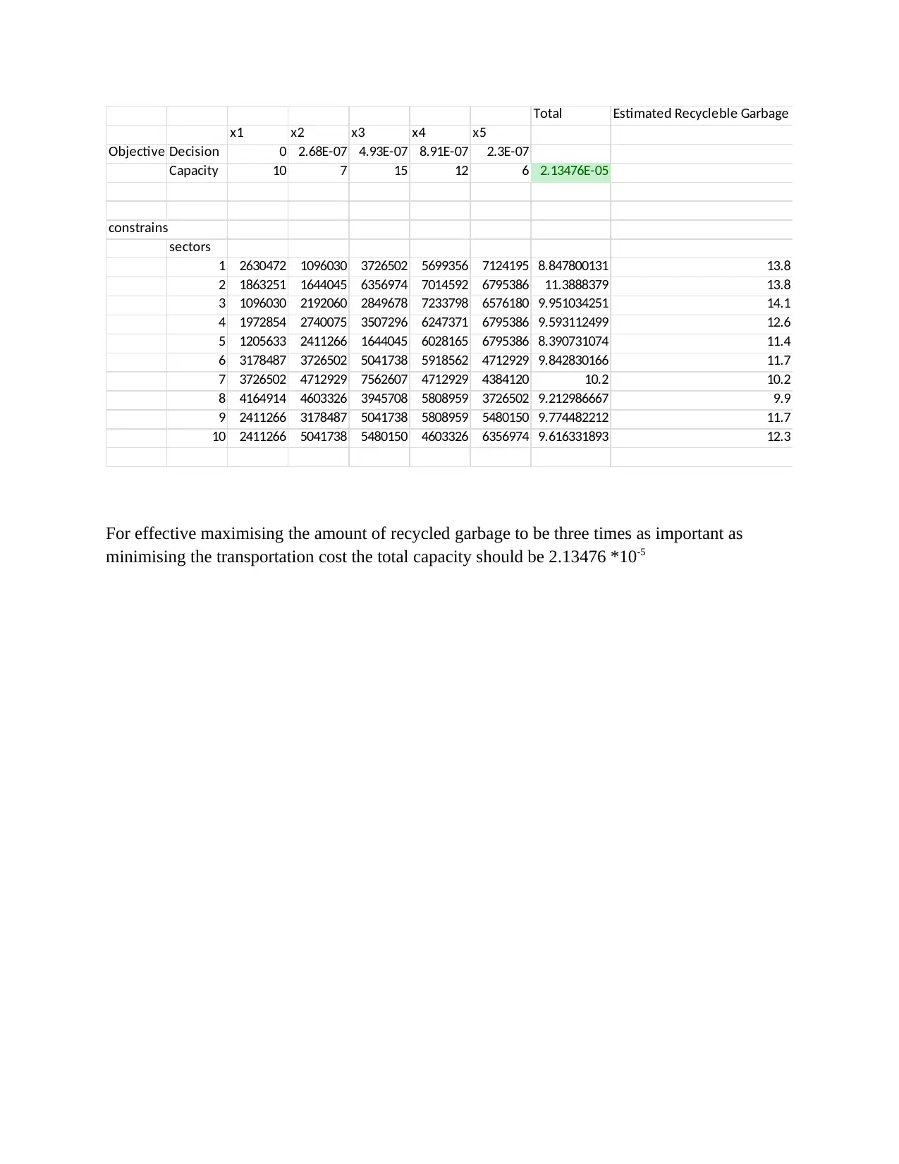
Total Estimated Recycleble Garbage
x1 x2 x3 x4 x5
Objective Decision 0 2.68E-07 4.93E-07 8.91E-07 2.3E-07
Capacity 10 7 15 12 6 2.13476E-05
constrains
sectors
1 2630472 1096030 3726502 5699356 7124195 8.847800131 13.8
2 1863251 1644045 6356974 7014592 6795386 11.3888379 13.8
3 1096030 2192060 2849678 7233798 6576180 9.951034251 14.1
4 1972854 2740075 3507296 6247371 6795386 9.593112499 12.6
5 1205633 2411266 1644045 6028165 6795386 8.390731074 11.4
6 3178487 3726502 5041738 5918562 4712929 9.842830166 11.7
7 3726502 4712929 7562607 4712929 4384120 10.2 10.2
8 4164914 4603326 3945708 5808959 3726502 9.212986667 9.9
9 2411266 3178487 5041738 5808959 5480150 9.774482212 11.7
10 2411266 5041738 5480150 4603326 6356974 9.616331893 12.3
For effective maximising the amount of recycled garbage to be three times as important as
minimising the transportation cost the total capacity should be 2.13476 *10-5
Secure Best Marks with AI Grader
Need help grading? Try our AI Grader for instant feedback on your assignments.
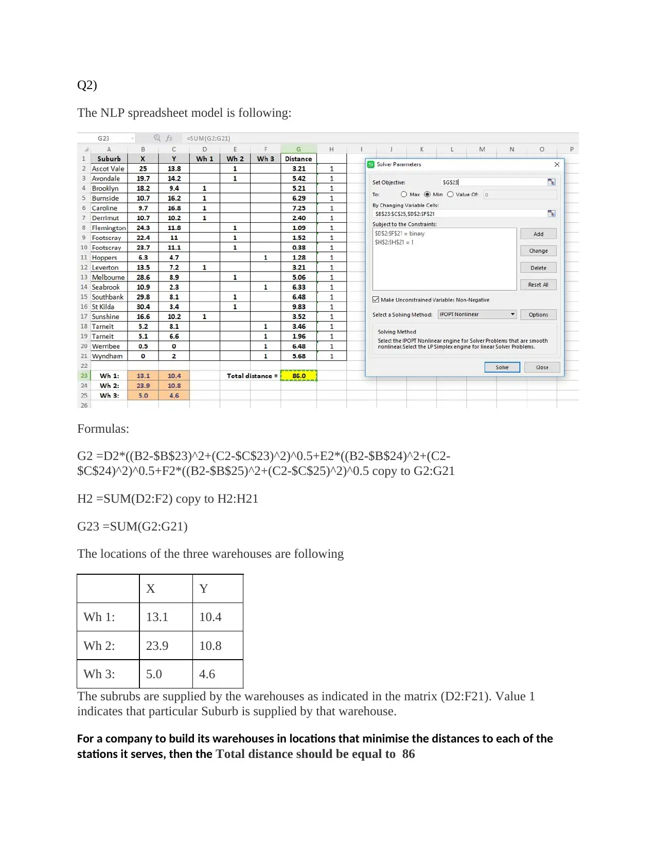
Q2)
The NLP spreadsheet model is following:
Formulas:
G2 =D2*((B2-$B$23)^2+(C2-$C$23)^2)^0.5+E2*((B2-$B$24)^2+(C2-
$C$24)^2)^0.5+F2*((B2-$B$25)^2+(C2-$C$25)^2)^0.5 copy to G2:G21
H2 =SUM(D2:F2) copy to H2:H21
G23 =SUM(G2:G21)
The locations of the three warehouses are following
X Y
Wh 1: 13.1 10.4
Wh 2: 23.9 10.8
Wh 3: 5.0 4.6
The subrubs are supplied by the warehouses as indicated in the matrix (D2:F21). Value 1
indicates that particular Suburb is supplied by that warehouse.
For a company to build its warehouses in locations that minimise the distances to each of the
stations it serves, then the Total distance should be equal to 86
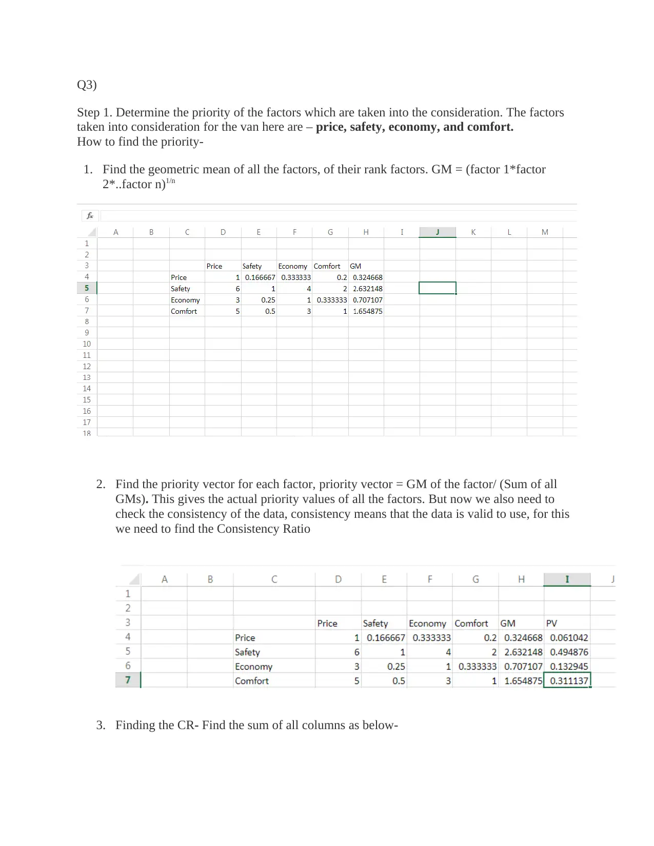
Q3)
Step 1. Determine the priority of the factors which are taken into the consideration. The factors
taken into consideration for the van here are – price, safety, economy, and comfort.
How to find the priority-
1. Find the geometric mean of all the factors, of their rank factors. GM = (factor 1*factor
2*..factor n)1/n
2. Find the priority vector for each factor, priority vector = GM of the factor/ (Sum of all
GMs). This gives the actual priority values of all the factors. But now we also need to
check the consistency of the data, consistency means that the data is valid to use, for this
we need to find the Consistency Ratio
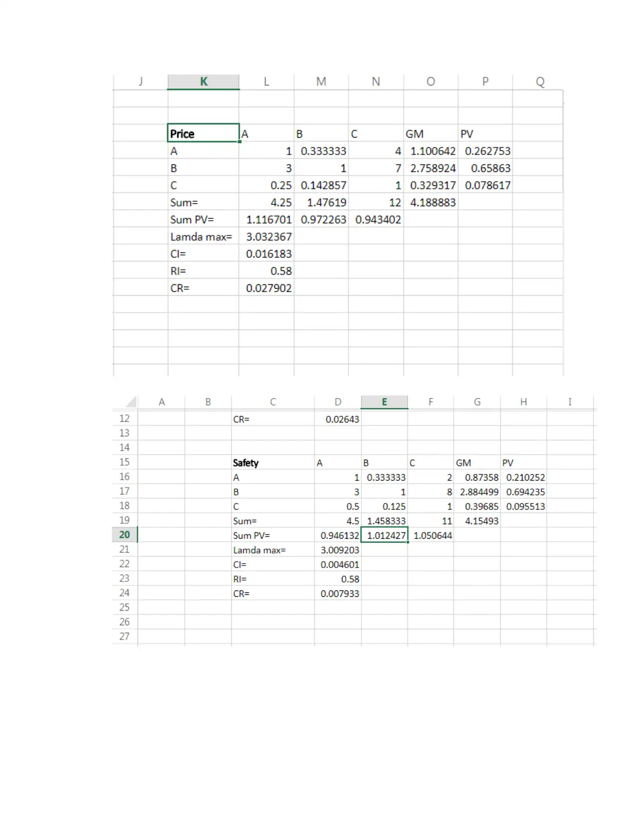
3. Finding the CR- Find the sum of all columns as below-
Step 1. Determine the priority of the factors which are taken into the consideration. The factors
taken into consideration for the van here are – price, safety, economy, and comfort.
How to find the priority-
1. Find the geometric mean of all the factors, of their rank factors. GM = (factor 1*factor
2*..factor n)1/n
2. Find the priority vector for each factor, priority vector = GM of the factor/ (Sum of all
GMs). This gives the actual priority values of all the factors. But now we also need to
check the consistency of the data, consistency means that the data is valid to use, for this
we need to find the Consistency Ratio
3. Finding the CR- Find the sum of all columns as below-
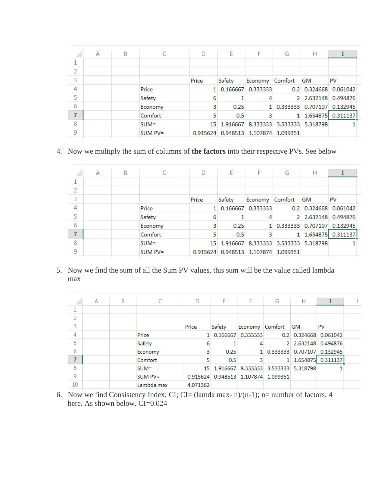
4. Now we multiply the sum of columns of the factors into their respective PVs. See below
5. Now we find the sum of all the Sum PV values, this sum will be the value called lambda
max
6. Now we find Consistency Index; CI; CI= (lamda max- n)/(n-1); n= number of factors; 4
here. As shown below. CI=0.024
5. Now we find the sum of all the Sum PV values, this sum will be the value called lambda
max
6. Now we find Consistency Index; CI; CI= (lamda max- n)/(n-1); n= number of factors; 4
here. As shown below. CI=0.024
Paraphrase This Document
Need a fresh take? Get an instant paraphrase of this document with our AI Paraphraser
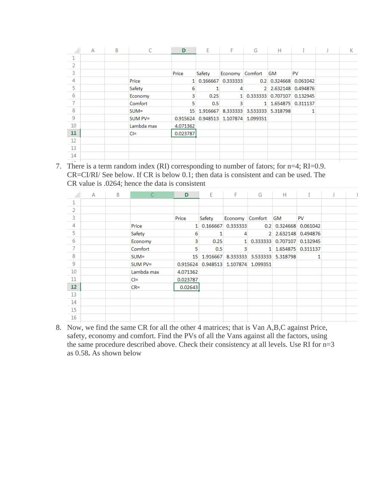
7. There is a term random index (RI) corresponding to number of fators; for n=4; RI=0.9.
CR=CI/RI/ See below. If CR is below 0.1; then data is consistent and can be used. The
CR value is .0264; hence the data is consistent
8. Now, we find the same CR for all the other 4 matrices; that is Van A,B,C against Price,
safety, economy and comfort. Find the PVs of all the Vans against all the factors, using
the same procedure described above. Check their consistency at all levels. Use RI for n=3
as 0.58. As shown below
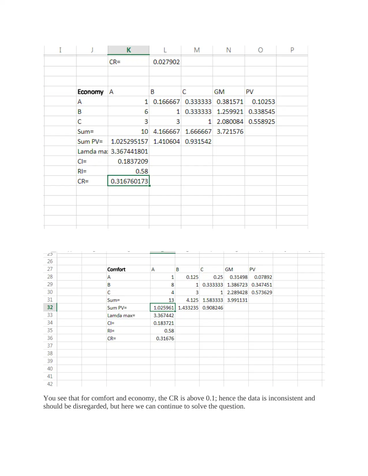
You see that for comfort and economy, the CR is above 0.1; hence the data is inconsistent and
should be disregarded, but here we can continue to solve the question.
should be disregarded, but here we can continue to solve the question.
Secure Best Marks with AI Grader
Need help grading? Try our AI Grader for instant feedback on your assignments.
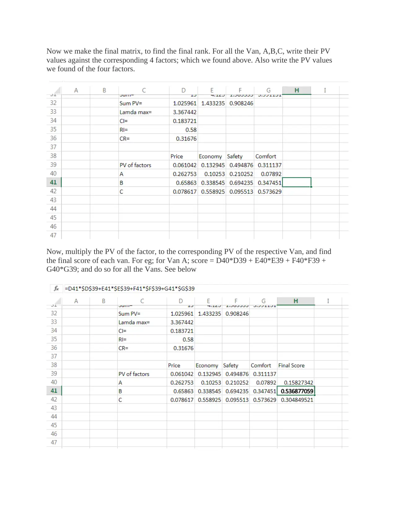
Now we make the final matrix, to find the final rank. For all the Van, A,B,C, write their PV
values against the corresponding 4 factors; which we found above. Also write the PV values
we found of the four factors.
Now, multiply the PV of the factor, to the corresponding PV of the respective Van, and find
the final score of each van. For eg; for Van A; score = D40*D39 + E40*E39 + F40*F39 +
G40*G39; and do so for all the Vans. See below
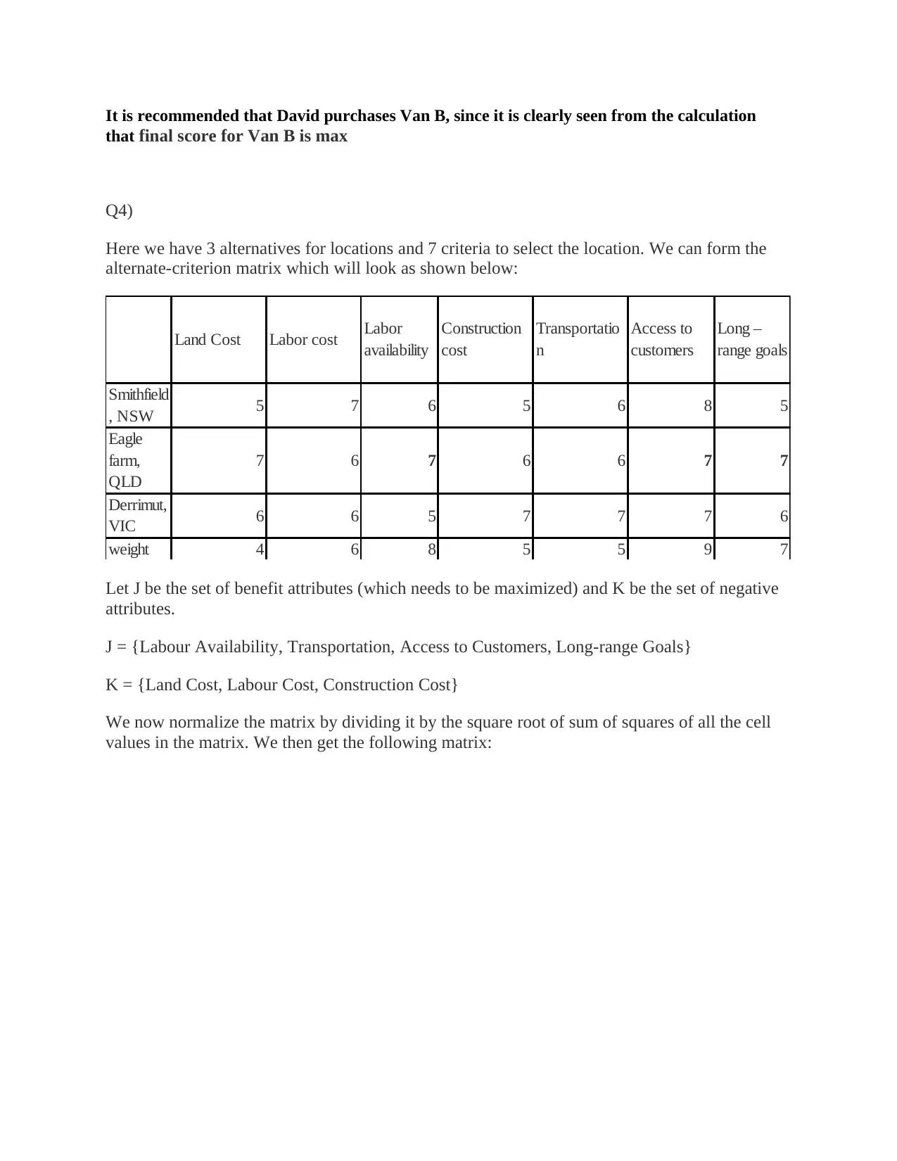
It is recommended that David purchases Van B, since it is clearly seen from the calculation
that final score for Van B is max
Q4)
Here we have 3 alternatives for locations and 7 criteria to select the location. We can form the
alternate-criterion matrix which will look as shown below:
Land Cost Labor cost Labor
availability
Construction
cost
Transportatio
n
Access to
customers
Long –
range goals
Smithfield
, NSW 5 7 6 5 6 8 5
Eagle
farm,
QLD
7 6 7 6 6 7 7
Derrimut,
VIC 6 6 5 7 7 7 6
weight 4 6 8 5 5 9 7
Let J be the set of benefit attributes (which needs to be maximized) and K be the set of negative
attributes.
J = {Labour Availability, Transportation, Access to Customers, Long-range Goals}
K = {Land Cost, Labour Cost, Construction Cost}
We now normalize the matrix by dividing it by the square root of sum of squares of all the cell
values in the matrix. We then get the following matrix:
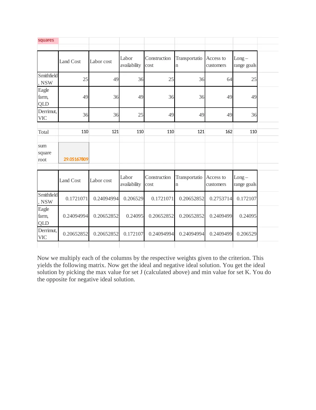
squares
Land Cost Labor cost Labor
availability
Construction
cost
Transportatio
n
Access to
customers
Long –
range goals
Smithfield
, NSW 25 49 36 25 36 64 25
Eagle
farm,
QLD
49 36 49 36 36 49 49
Derrimut,
VIC 36 36 25 49 49 49 36
Total 110 121 110 110 121 162 110
sum
square
root 29.05167809
Land Cost Labor cost Labor
availability
Construction
cost
Transportatio
n
Access to
customers
Long –
range goals
Smithfield
, NSW 0.1721071 0.24094994 0.206529 0.1721071 0.20652852 0.2753714 0.172107
Eagle
farm,
QLD
0.24094994 0.20652852 0.24095 0.20652852 0.20652852 0.2409499 0.24095
Derrimut,
VIC 0.20652852 0.20652852 0.172107 0.24094994 0.24094994 0.2409499 0.206529
Now we multiply each of the columns by the respective weights given to the criterion. This
yields the following matrix. Now get the ideal and negative ideal solution. You get the ideal
solution by picking the max value for set J (calculated above) and min value for set K. You do
the opposite for negative ideal solution.
Land Cost Labor cost Labor
availability
Construction
cost
Transportatio
n
Access to
customers
Long –
range goals
Smithfield
, NSW 25 49 36 25 36 64 25
Eagle
farm,
QLD
49 36 49 36 36 49 49
Derrimut,
VIC 36 36 25 49 49 49 36
Total 110 121 110 110 121 162 110
sum
square
root 29.05167809
Land Cost Labor cost Labor
availability
Construction
cost
Transportatio
n
Access to
customers
Long –
range goals
Smithfield
, NSW 0.1721071 0.24094994 0.206529 0.1721071 0.20652852 0.2753714 0.172107
Eagle
farm,
QLD
0.24094994 0.20652852 0.24095 0.20652852 0.20652852 0.2409499 0.24095
Derrimut,
VIC 0.20652852 0.20652852 0.172107 0.24094994 0.24094994 0.2409499 0.206529
Now we multiply each of the columns by the respective weights given to the criterion. This
yields the following matrix. Now get the ideal and negative ideal solution. You get the ideal
solution by picking the max value for set J (calculated above) and min value for set K. You do
the opposite for negative ideal solution.
Paraphrase This Document
Need a fresh take? Get an instant paraphrase of this document with our AI Paraphraser
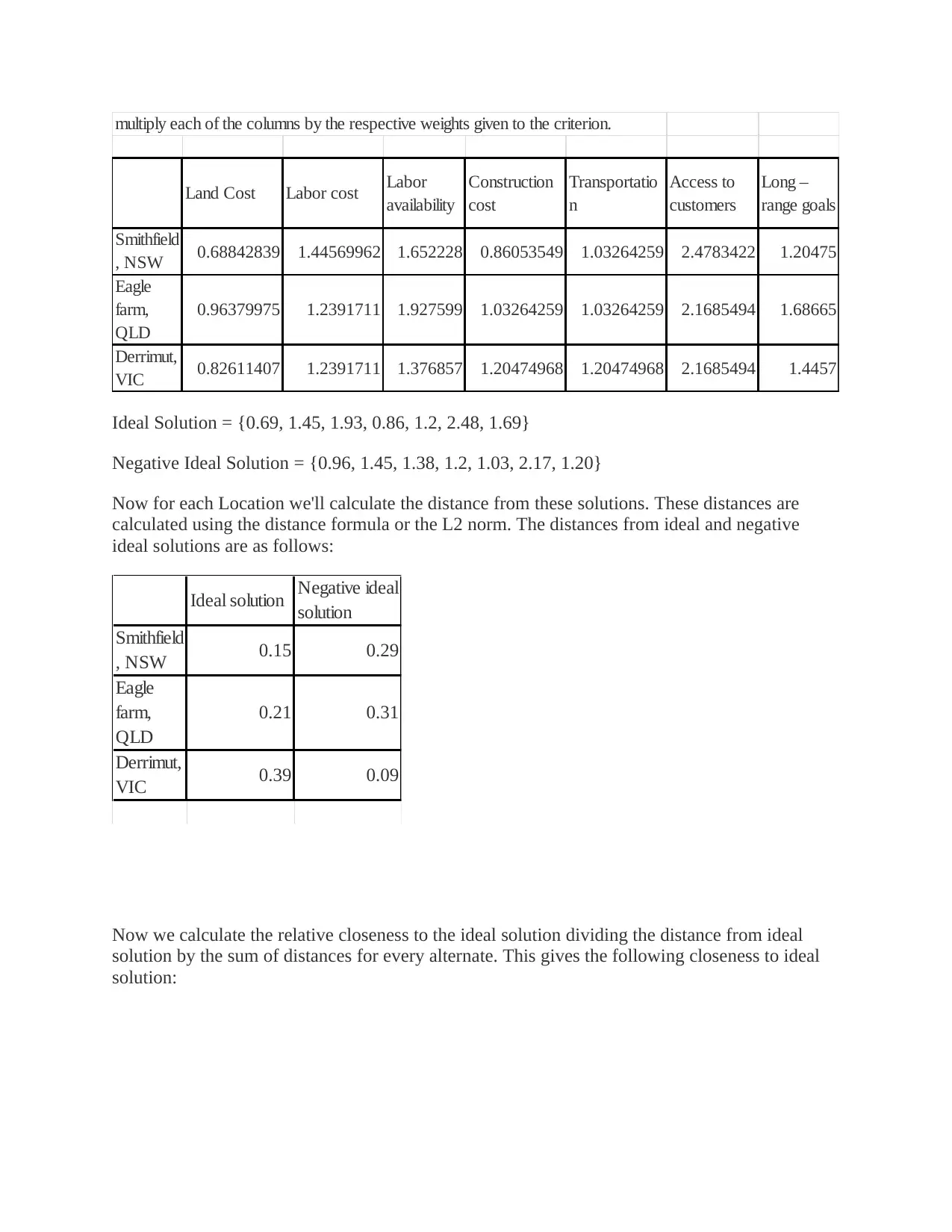
multiply each of the columns by the respective weights given to the criterion.
Land Cost Labor cost Labor
availability
Construction
cost
Transportatio
n
Access to
customers
Long –
range goals
Smithfield
, NSW 0.68842839 1.44569962 1.652228 0.86053549 1.03264259 2.4783422 1.20475
Eagle
farm,
QLD
0.96379975 1.2391711 1.927599 1.03264259 1.03264259 2.1685494 1.68665
Derrimut,
VIC 0.82611407 1.2391711 1.376857 1.20474968 1.20474968 2.1685494 1.4457
Ideal Solution = {0.69, 1.45, 1.93, 0.86, 1.2, 2.48, 1.69}
Negative Ideal Solution = {0.96, 1.45, 1.38, 1.2, 1.03, 2.17, 1.20}
Now for each Location we'll calculate the distance from these solutions. These distances are
calculated using the distance formula or the L2 norm. The distances from ideal and negative
ideal solutions are as follows:
Ideal solution Negative ideal
solution
Smithfield
, NSW 0.15 0.29
Eagle
farm,
QLD
0.21 0.31
Derrimut,
VIC 0.39 0.09
Now we calculate the relative closeness to the ideal solution dividing the distance from ideal
solution by the sum of distances for every alternate. This gives the following closeness to ideal
solution:
Land Cost Labor cost Labor
availability
Construction
cost
Transportatio
n
Access to
customers
Long –
range goals
Smithfield
, NSW 0.68842839 1.44569962 1.652228 0.86053549 1.03264259 2.4783422 1.20475
Eagle
farm,
QLD
0.96379975 1.2391711 1.927599 1.03264259 1.03264259 2.1685494 1.68665
Derrimut,
VIC 0.82611407 1.2391711 1.376857 1.20474968 1.20474968 2.1685494 1.4457
Ideal Solution = {0.69, 1.45, 1.93, 0.86, 1.2, 2.48, 1.69}
Negative Ideal Solution = {0.96, 1.45, 1.38, 1.2, 1.03, 2.17, 1.20}
Now for each Location we'll calculate the distance from these solutions. These distances are
calculated using the distance formula or the L2 norm. The distances from ideal and negative
ideal solutions are as follows:
Ideal solution Negative ideal
solution
Smithfield
, NSW 0.15 0.29
Eagle
farm,
QLD
0.21 0.31
Derrimut,
VIC 0.39 0.09
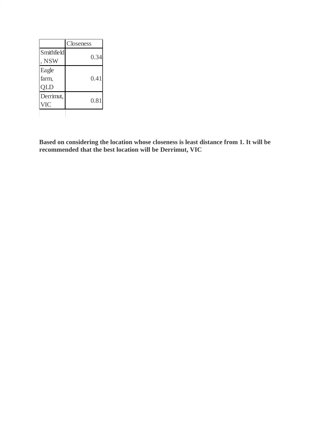
Now we calculate the relative closeness to the ideal solution dividing the distance from ideal
solution by the sum of distances for every alternate. This gives the following closeness to ideal
solution:
Closeness
Smithfield
, NSW 0.34
Eagle
farm,
QLD
0.41
Derrimut,
VIC 0.81
Based on considering the location whose closeness is least distance from 1. It will be
recommended that the best location will be Derrimut, VIC
Smithfield
, NSW 0.34
Eagle
farm,
QLD
0.41
Derrimut,
VIC 0.81
Based on considering the location whose closeness is least distance from 1. It will be
recommended that the best location will be Derrimut, VIC
1 out of 15
Related Documents


Your All-in-One AI-Powered Toolkit for Academic Success.
+13062052269
info@desklib.com
Available 24*7 on WhatsApp / Email
![[object Object]](/_next/static/media/star-bottom.7253800d.svg)
Unlock your academic potential
© 2024 | Zucol Services PVT LTD | All rights reserved.