Statistics Study Material

Get access to study material for statistics including solved assignments, essays, dissertations, and more. Improve your understanding of statistics with Desklib.

STATISTICS

Question 2:
a. Provide a 95% confidence interval for all the patients who are referred to
the health centre by the hospital.
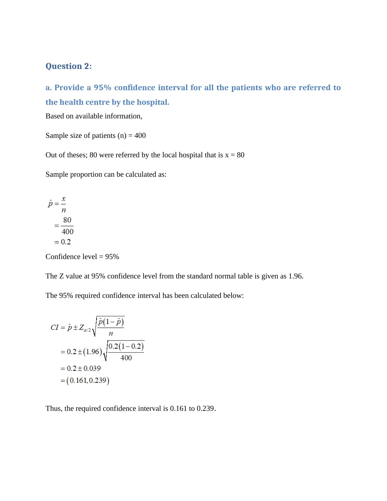
Based on available information,
Sample size of patients (n) = 400
Out of theses; 80 were referred by the local hospital that is x = 80
Sample proportion can be calculated as:
Confidence level = 95%
The Z value at 95% confidence level from the standard normal table is given as 1.96.
The 95% required confidence interval has been calculated below:
Thus, the required confidence interval is 0.161 to 0.239.

b. What sample size would be required to estimate the proportion of all
hospital referrals to the health centre with a margin of error of 0.04 or less at
95% confidence?
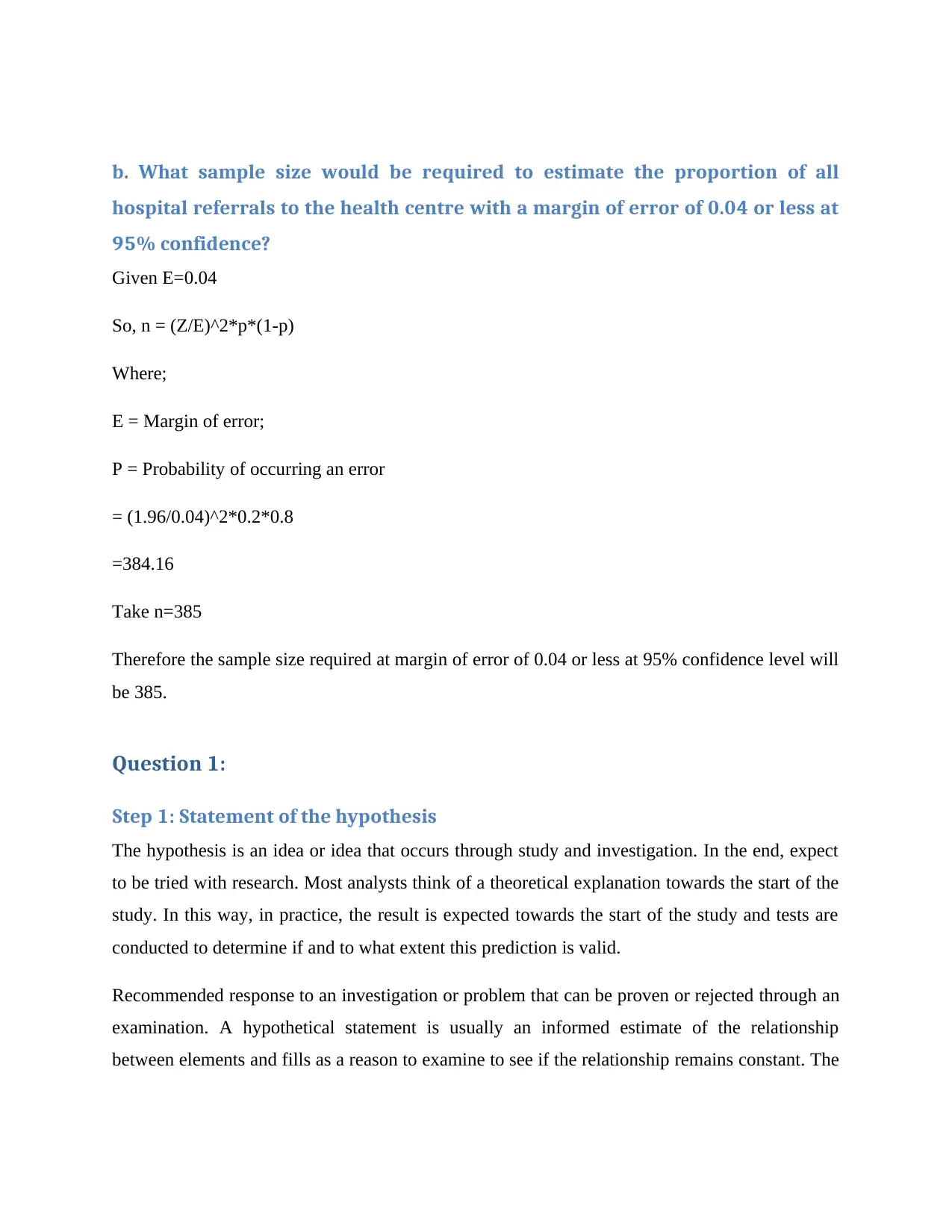
Given E=0.04
So, n = (Z/E)^2*p*(1-p)
Where;
E = Margin of error;
P = Probability of occurring an error
= (1.96/0.04)^2*0.2*0.8
=384.16
Take n=385
Therefore the sample size required at margin of error of 0.04 or less at 95% confidence level will
be 385.
Question 1:
Step 1: Statement of the hypothesis
The hypothesis is an idea or idea that occurs through study and investigation. In the end, expect
to be tried with research. Most analysts think of a theoretical explanation towards the start of the
study. In this way, in practice, the result is expected towards the start of the study and tests are
conducted to determine if and to what extent this prediction is valid.
Recommended response to an investigation or problem that can be proven or rejected through an
examination. A hypothetical statement is usually an informed estimate of the relationship
between elements and fills as a reason to examine to see if the relationship remains constant. The

genres are extracted in the business process development activities to perform a study that
determines the best combination of variables for a procedure.
The research hypothesis (H1) is the news made by experts when they theorize the results of a
study or study.
The hypothesis is realized through a variety of means, but it is usually the result of a thought
process in which ideas lead to a hypothetical arrangement. Researchers at that level use a large
set of subtraction strategies to demonstrate viable, tangible and realistic profitability.
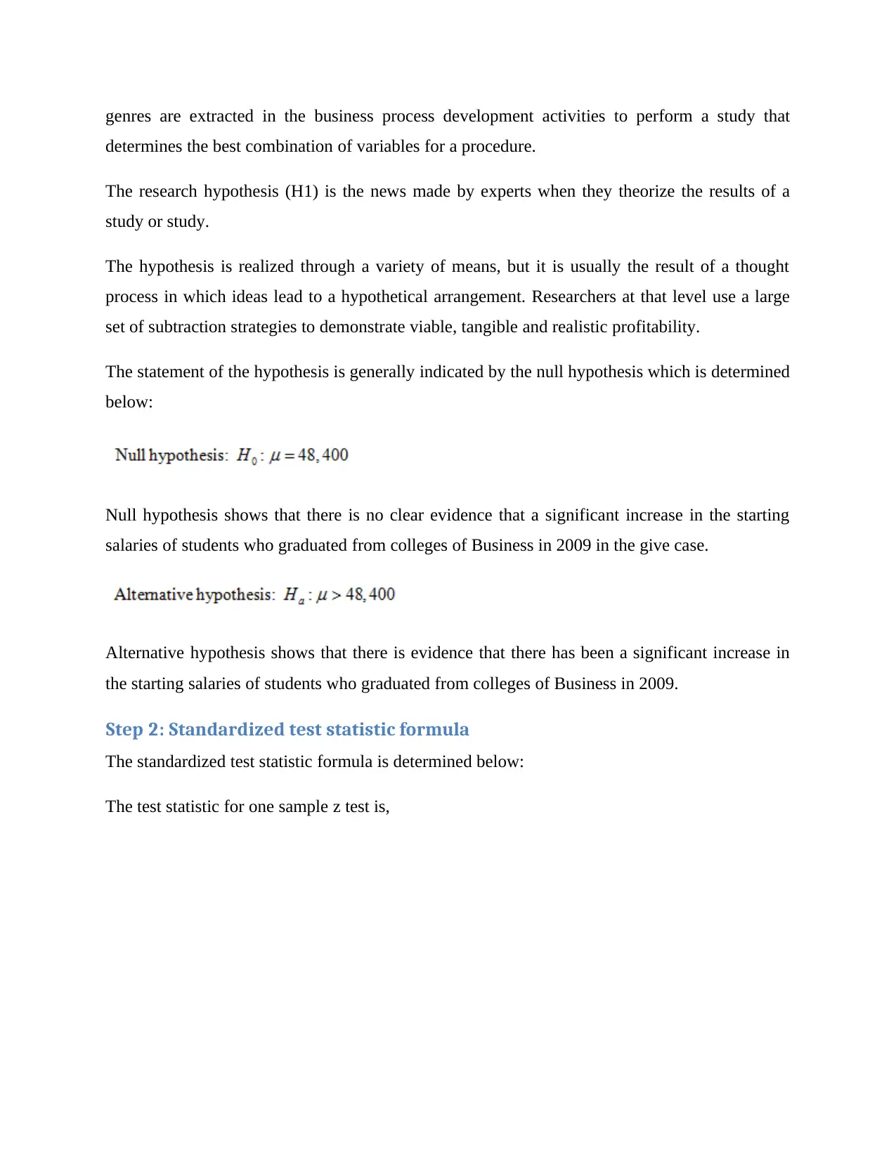
The statement of the hypothesis is generally indicated by the null hypothesis which is determined
below:
Null hypothesis shows that there is no clear evidence that a significant increase in the starting
salaries of students who graduated from colleges of Business in 2009 in the give case.
Alternative hypothesis shows that there is evidence that there has been a significant increase in
the starting salaries of students who graduated from colleges of Business in 2009.
Step 2: Standardized test statistic formula
The standardized test statistic formula is determined below:
The test statistic for one sample z test is,

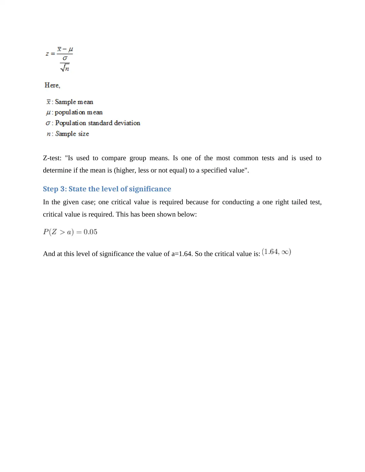
Z-test: "Is used to compare group means. Is one of the most common tests and is used to
determine if the mean is (higher, less or not equal) to a specified value".
Step 3: State the level of significance
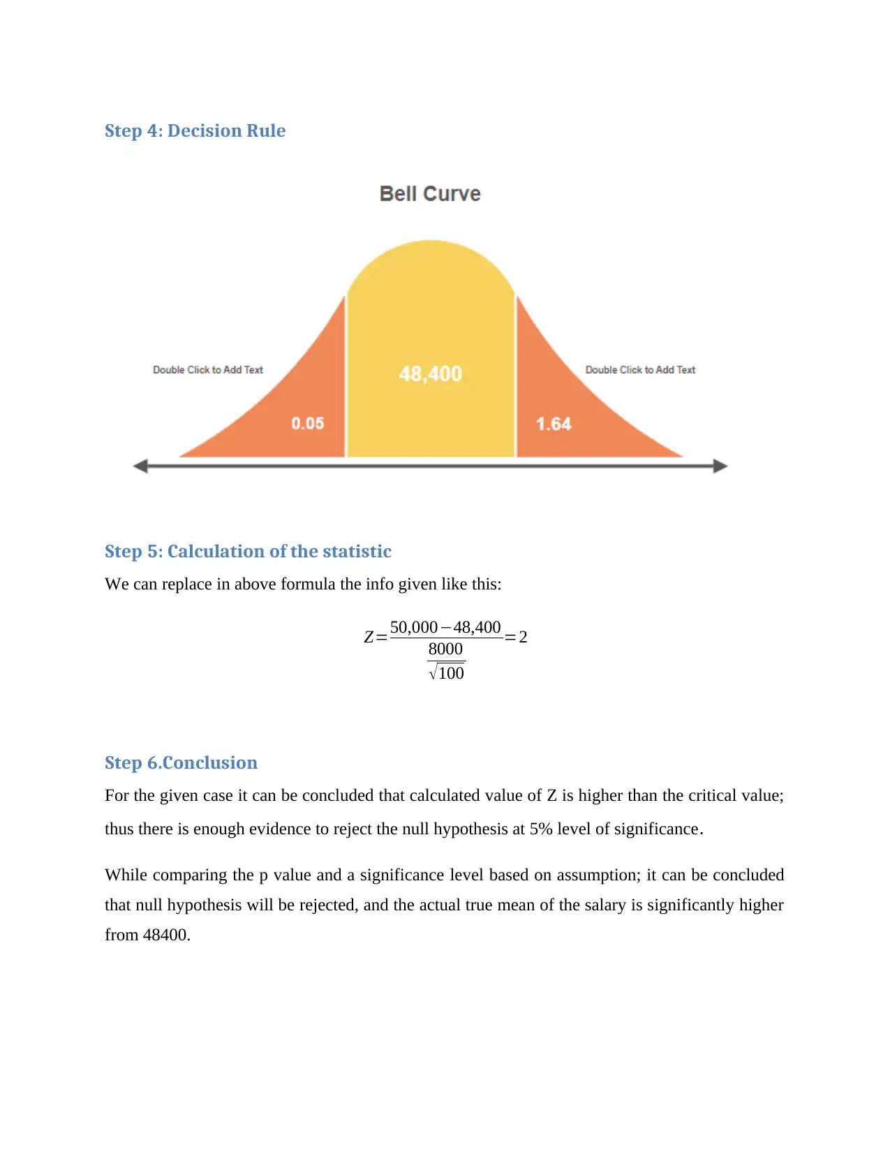
In the given case; one critical value is required because for conducting a one right tailed test,
critical value is required. This has been shown below:
And at this level of significance the value of a=1.64. So the critical value is:

Step 4: Decision Rule
Step 5: Calculation of the statistic
We can replace in above formula the info given like this:
Z=50,000−48,400
8000
√ 100
=2
Step 6.Conclusion
For the given case it can be concluded that calculated value of Z is higher than the critical value;
thus there is enough evidence to reject the null hypothesis at 5% level of significance.
While comparing the p value and a significance level based on assumption; it can be concluded
that null hypothesis will be rejected, and the actual true mean of the salary is significantly higher
from 48400.

Question 3:
a. State the null and alternative hypothesis for single factor ANOVA.
Hypothesis:
H0: Mean is same for all groups;
H1: Mean is not same for all groups
b. State the decision rule ( =0.05).α
Decision rule:
If p-value is equal to or greater than level of significance, then fail to reject the null hypothesis.
If p-value is less than level of significance, then reject the null hypothesis.
c. Calculate the test statistic.
Consider the level of significance as 0.05.
Step by step procedure to find missing values using EXCEL:
In Excel sheet, enter Process 1, Process 2 and Process 3 in different columns.
In Data, select Data Analysis and Choose Anova: Single Factor.
In Input Range, select Process 1, Process 2 and Process 3.
Click Labels in First Row.
Enter α =0.05
Click OK.
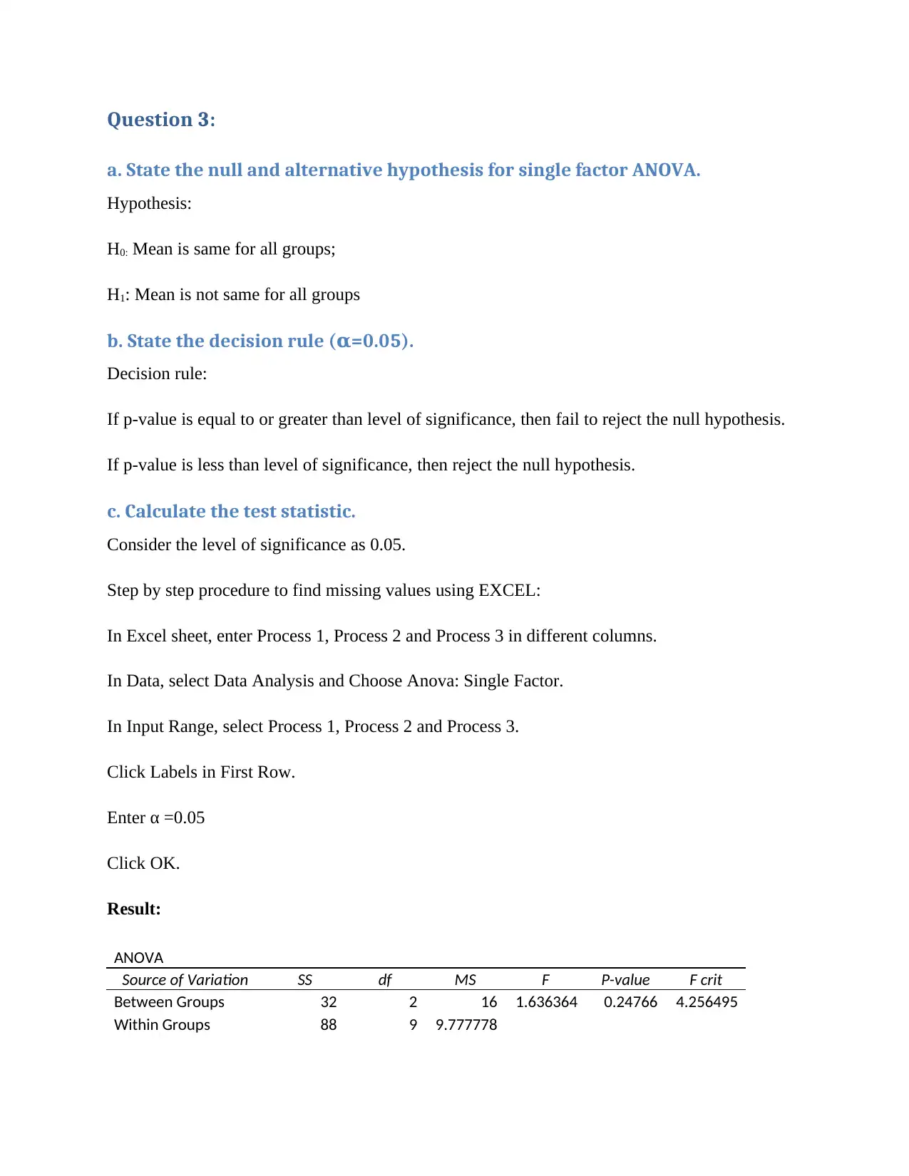
Result:
ANOVA
Source of Variation SS df MS F P-value F crit
Between Groups 32 2 16 1.636364 0.24766 4.256495
Within Groups 88 9 9.777778

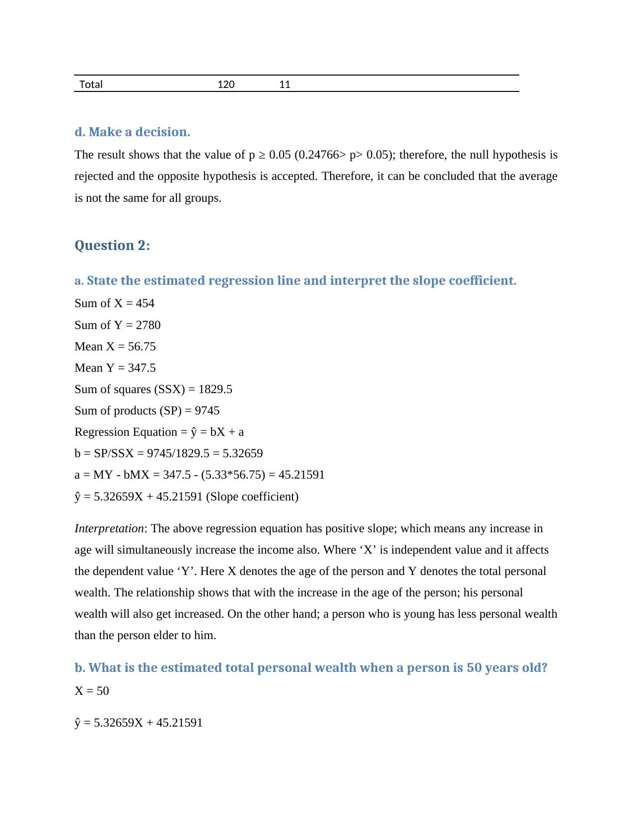
Total 120 11
d. Make a decision.
The result shows that the value of p ≥ 0.05 (0.24766> p> 0.05); therefore, the null hypothesis is
rejected and the opposite hypothesis is accepted. Therefore, it can be concluded that the average
is not the same for all groups.
Question 2:
a. State the estimated regression line and interpret the slope coefficient.
Sum of X = 454
Sum of Y = 2780
Mean X = 56.75
Mean Y = 347.5
Sum of squares (SSX) = 1829.5
Sum of products (SP) = 9745
Regression Equation = ŷ = bX + a
b = SP/SSX = 9745/1829.5 = 5.32659
a = MY - bMX = 347.5 - (5.33*56.75) = 45.21591
ŷ = 5.32659X + 45.21591 (Slope coefficient)
Interpretation: The above regression equation has positive slope; which means any increase in
age will simultaneously increase the income also. Where ‘X’ is independent value and it affects
the dependent value ‘Y’. Here X denotes the age of the person and Y denotes the total personal
wealth. The relationship shows that with the increase in the age of the person; his personal
wealth will also get increased. On the other hand; a person who is young has less personal wealth
than the person elder to him.
b. What is the estimated total personal wealth when a person is 50 years old?
X = 50
ŷ = 5.32659X + 45.21591

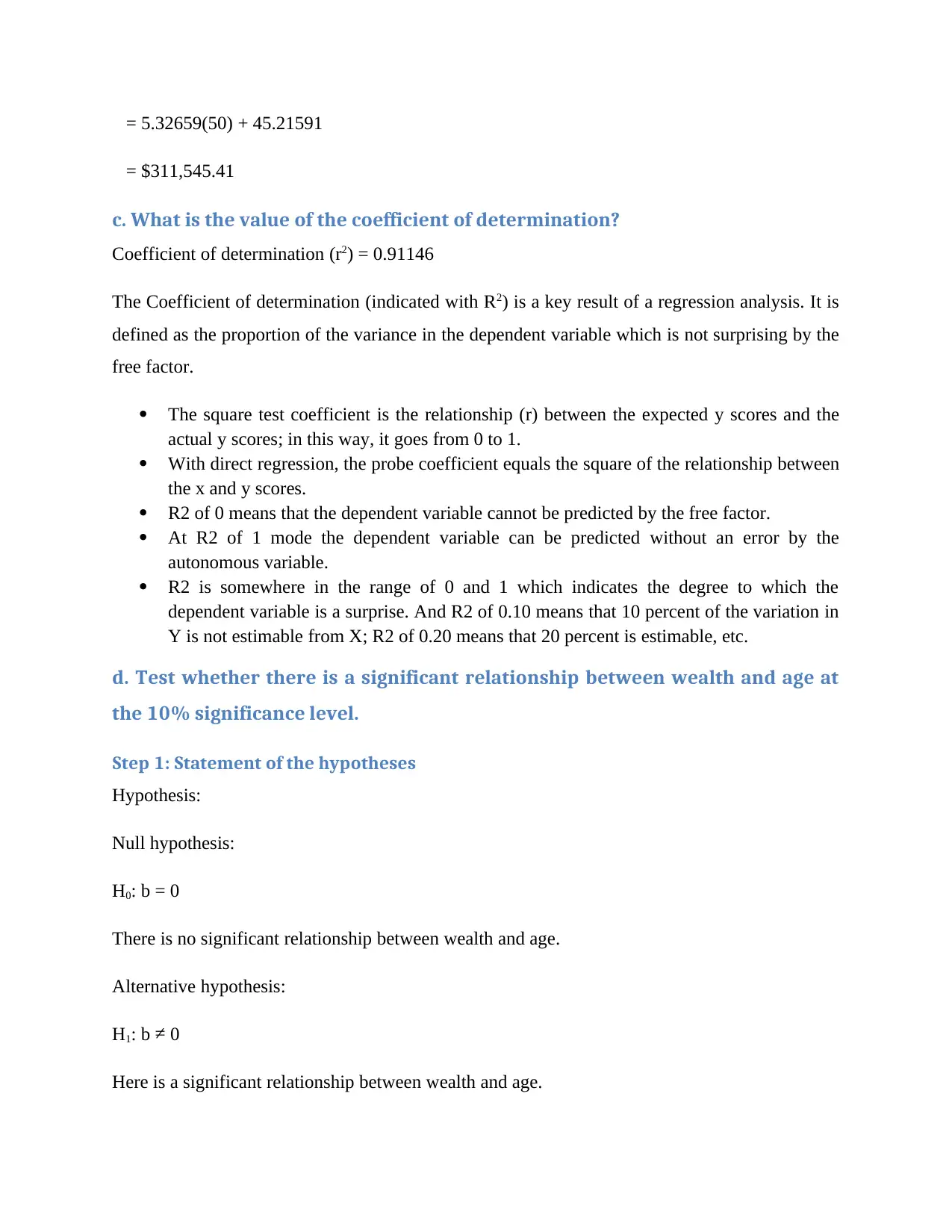
= 5.32659(50) + 45.21591
= $311,545.41
c. What is the value of the coefficient of determination?
Coefficient of determination (r2) = 0.91146
The Coefficient of determination (indicated with R2) is a key result of a regression analysis. It is
defined as the proportion of the variance in the dependent variable which is not surprising by the
free factor.
 The square test coefficient is the relationship (r) between the expected y scores and the
actual y scores; in this way, it goes from 0 to 1.
 With direct regression, the probe coefficient equals the square of the relationship between
the x and y scores.
 R2 of 0 means that the dependent variable cannot be predicted by the free factor.
 At R2 of 1 mode the dependent variable can be predicted without an error by the
autonomous variable.
 R2 is somewhere in the range of 0 and 1 which indicates the degree to which the
dependent variable is a surprise. And R2 of 0.10 means that 10 percent of the variation in
Y is not estimable from X; R2 of 0.20 means that 20 percent is estimable, etc.
d. Test whether there is a significant relationship between wealth and age at
the 10% significance level.
Step 1: Statement of the hypotheses
Hypothesis:
Null hypothesis:
H0: b = 0
There is no significant relationship between wealth and age.
Alternative hypothesis:
H1: b ≠ 0
Here is a significant relationship between wealth and age.

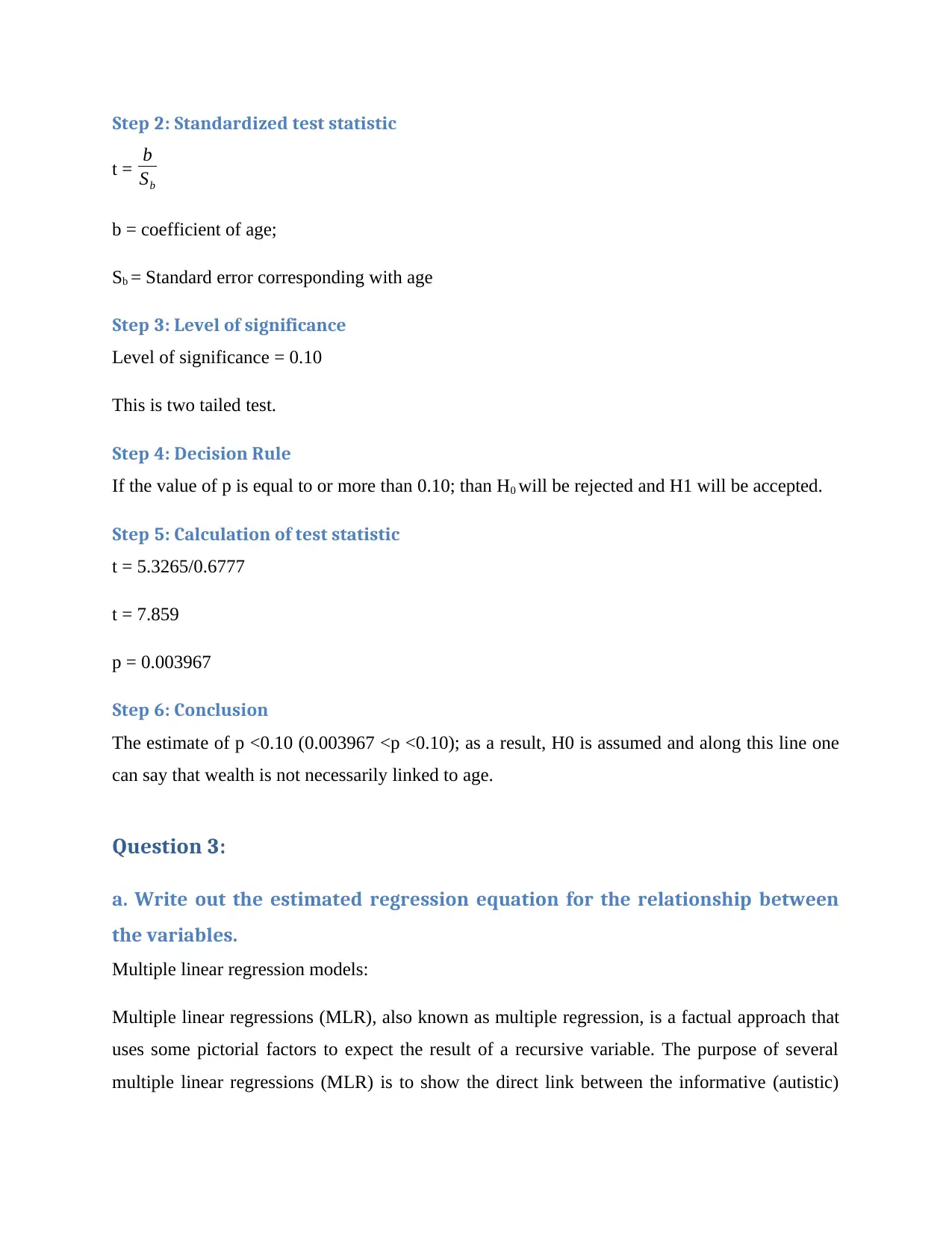
Step 2: Standardized test statistic
t = b
Sb
b = coefficient of age;
Sb = Standard error corresponding with age
Step 3: Level of significance
Level of significance = 0.10
This is two tailed test.
Step 4: Decision Rule
If the value of p is equal to or more than 0.10; than H0 will be rejected and H1 will be accepted.
Step 5: Calculation of test statistic
t = 5.3265/0.6777
t = 7.859
p = 0.003967
Step 6: Conclusion
The estimate of p <0.10 (0.003967 <p <0.10); as a result, H0 is assumed and along this line one
can say that wealth is not necessarily linked to age.
Question 3:
a. Write out the estimated regression equation for the relationship between
the variables.
Multiple linear regression models:
Multiple linear regressions (MLR), also known as multiple regression, is a factual approach that
uses some pictorial factors to expect the result of a recursive variable. The purpose of several
multiple linear regressions (MLR) is to show the direct link between the informative (autistic)

factors and a recursive (subordinate) variable. In general, a least squares normalized regression
for ordinary least-squares (OLS) are an array that contains more than one logical variable.
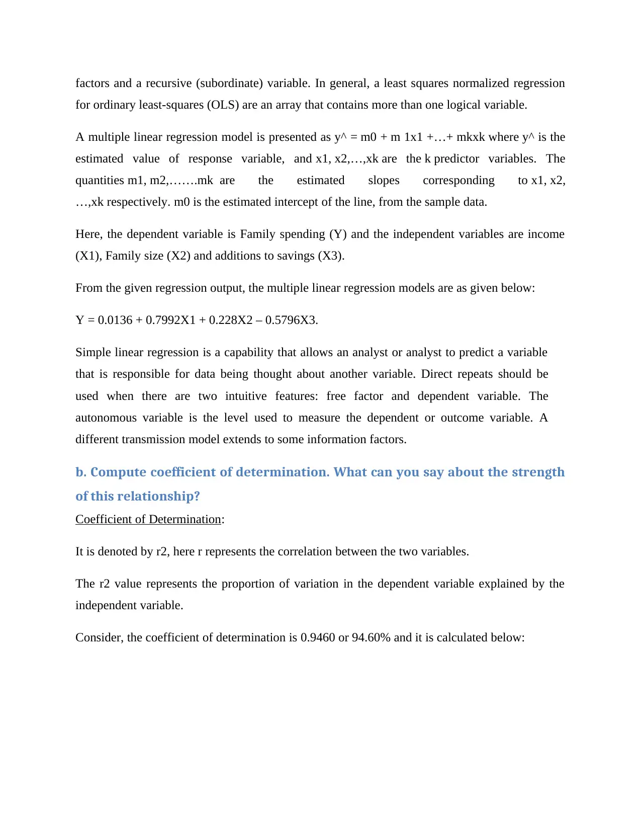
A multiple linear regression model is presented as y^ = m0 + m 1x1 +…+ mkxk where y^ is the
estimated value of response variable, and x1, x2,…,xk are the k predictor variables. The
quantities m1, m2,…….mk are the estimated slopes corresponding to x1, x2,
…,xk respectively. m0 is the estimated intercept of the line, from the sample data.
Here, the dependent variable is Family spending (Y) and the independent variables are income
(X1), Family size (X2) and additions to savings (X3).
From the given regression output, the multiple linear regression models are as given below:
Y = 0.0136 + 0.7992X1 + 0.228X2 – 0.5796X3.
Simple linear regression is a capability that allows an analyst or analyst to predict a variable
that is responsible for data being thought about another variable. Direct repeats should be
used when there are two intuitive features: free factor and dependent variable. The
autonomous variable is the level used to measure the dependent or outcome variable. A
different transmission model extends to some information factors.
b. Compute coefficient of determination. What can you say about the strength
of this relationship?
Coefficient of Determination:
It is denoted by r2, here r represents the correlation between the two variables.
The r2 value represents the proportion of variation in the dependent variable explained by the
independent variable.
Consider, the coefficient of determination is 0.9460 or 94.60% and it is calculated below:

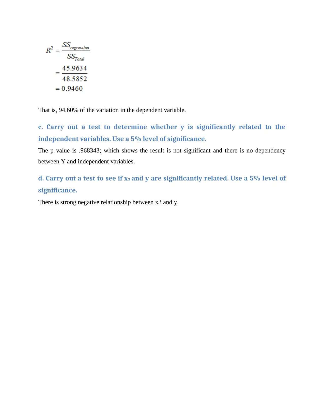
That is, 94.60% of the variation in the dependent variable.
c. Carry out a test to determine whether y is significantly related to the
independent variables. Use a 5% level of significance.
The p value is .968343; which shows the result is not significant and there is no dependency
between Y and independent variables.
d. Carry out a test to see if x3 and y are significantly related. Use a 5% level of
significance.
There is strong negative relationship between x3 and y.