Statistical Analysis of UK Netflix Viewers: Descriptive and Inferential Statistics

This coursework provides a statistical analysis of UK Netflix viewers using descriptive and inferential statistics. It includes mean, range, standard deviation, coefficient of variation, median, correlation matrix, regression equation, network diagram, critical path, and challenges faced during the analysis.

INDIVIDUAL
COURSEWORK

Table of Contents
TASK 1............................................................................................................................................3
1...................................................................................................................................................3
a)..................................................................................................................................................3
b)..................................................................................................................................................3
c)..................................................................................................................................................3
2...................................................................................................................................................4
TASK 2............................................................................................................................................4
1...................................................................................................................................................4
a) Table 1.....................................................................................................................................4
b) Table 2.....................................................................................................................................4
2...................................................................................................................................................5
3...................................................................................................................................................5
4...................................................................................................................................................5
TASK 3............................................................................................................................................6
1...................................................................................................................................................6
2...................................................................................................................................................7
3...................................................................................................................................................7
4...................................................................................................................................................7
TASK 4............................................................................................................................................8
1. Network diagram.....................................................................................................................8
2...................................................................................................................................................8
3...................................................................................................................................................8
TASK 5............................................................................................................................................9
1...................................................................................................................................................9
2...................................................................................................................................................9
3...................................................................................................................................................9
REFERENCES................................................................................................................................1

TASK 1
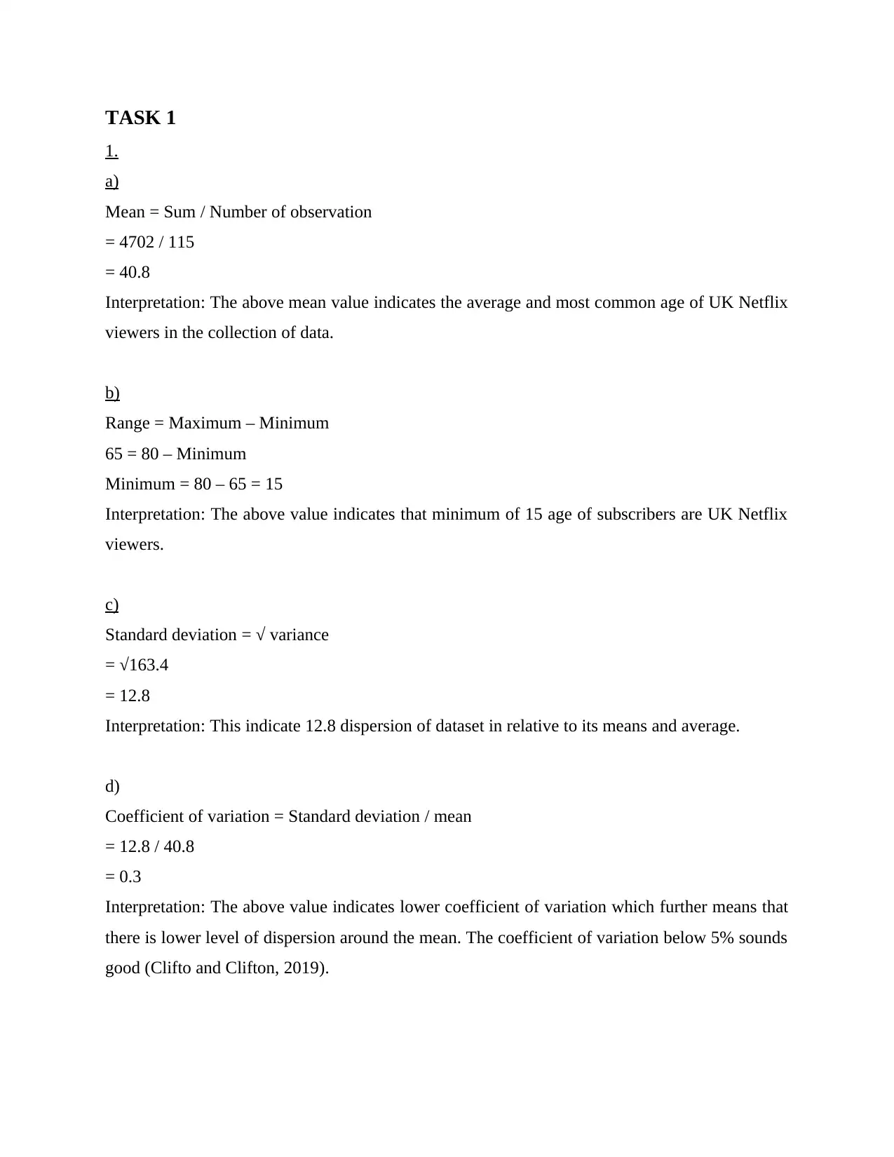
1.
a)
Mean = Sum / Number of observation
= 4702 / 115
= 40.8
Interpretation: The above mean value indicates the average and most common age of UK Netflix
viewers in the collection of data.
b)
Range = Maximum – Minimum
65 = 80 – Minimum
Minimum = 80 – 65 = 15
Interpretation: The above value indicates that minimum of 15 age of subscribers are UK Netflix
viewers.
c)
Standard deviation = √ variance
= √163.4
= 12.8
Interpretation: This indicate 12.8 dispersion of dataset in relative to its means and average.
d)
Coefficient of variation = Standard deviation / mean
= 12.8 / 40.8
= 0.3
Interpretation: The above value indicates lower coefficient of variation which further means that
there is lower level of dispersion around the mean. The coefficient of variation below 5% sounds
good (Clifto and Clifton, 2019).

2.
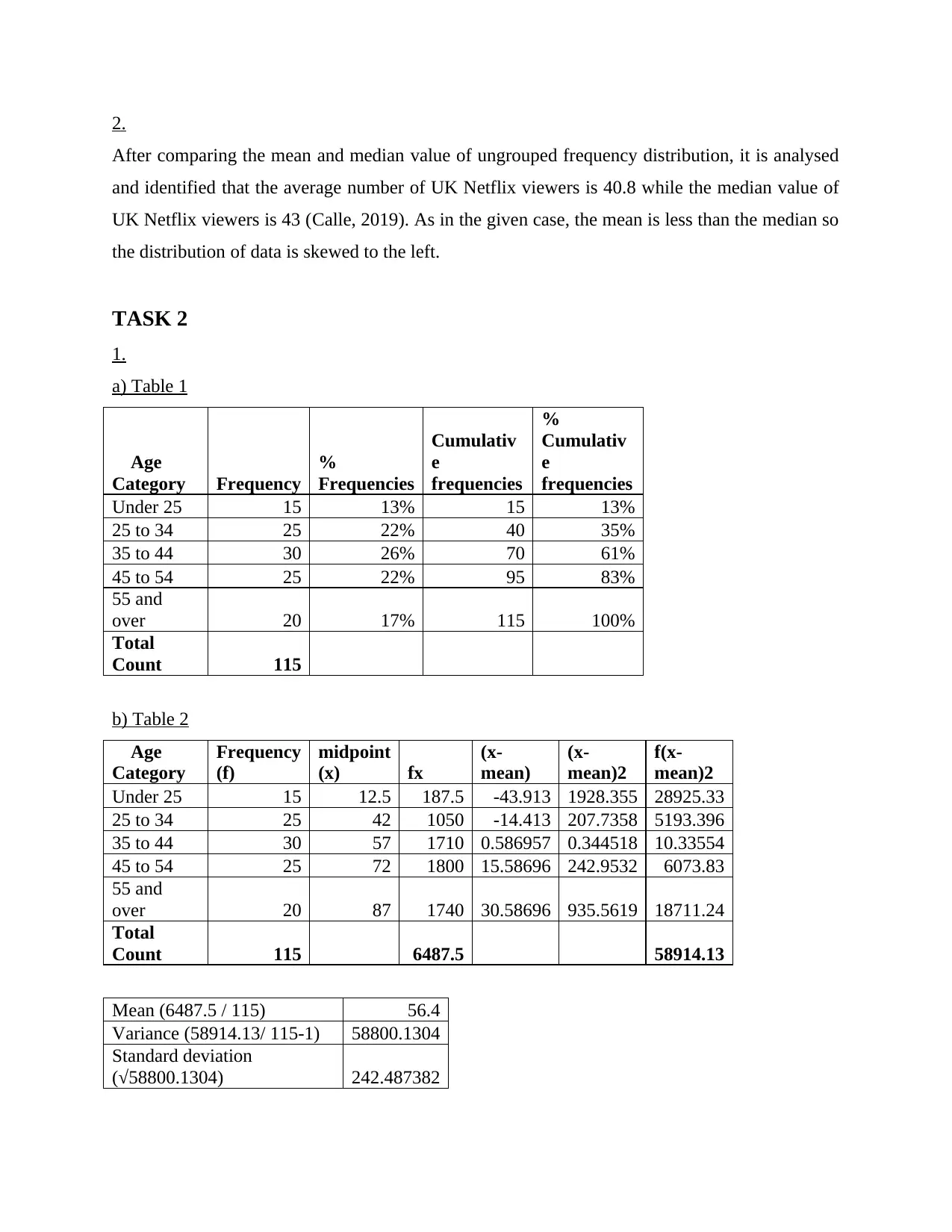
After comparing the mean and median value of ungrouped frequency distribution, it is analysed
and identified that the average number of UK Netflix viewers is 40.8 while the median value of
UK Netflix viewers is 43 (Calle, 2019). As in the given case, the mean is less than the median so
the distribution of data is skewed to the left.
TASK 2
1.
a) Table 1
Age
Category Frequency
%
Frequencies
Cumulativ
e
frequencies
%
Cumulativ
e
frequencies
Under 25 15 13% 15 13%
25 to 34 25 22% 40 35%
35 to 44 30 26% 70 61%
45 to 54 25 22% 95 83%
55 and
over 20 17% 115 100%
Total
Count 115
b) Table 2
Age
Category
Frequency
(f)
midpoint
(x) fx
(x-
mean)
(x-
mean)2
f(x-
mean)2
Under 25 15 12.5 187.5 -43.913 1928.355 28925.33
25 to 34 25 42 1050 -14.413 207.7358 5193.396
35 to 44 30 57 1710 0.586957 0.344518 10.33554
45 to 54 25 72 1800 15.58696 242.9532 6073.83
55 and
over 20 87 1740 30.58696 935.5619 18711.24
Total
Count 115 6487.5 58914.13
Mean (6487.5 / 115) 56.4
Variance (58914.13/ 115-1) 58800.1304
Standard deviation
(√58800.1304) 242.487382

2.
The mean and standard deviation calculated from raw data i.e., ungrouped data is more accurate
as compared to grouped data. It is because mean and standard deviation from grouped data is
computed based on assumption that all the observation within a class interval have a common
value equal to the mid-point of class interval. This includes some error.
3.
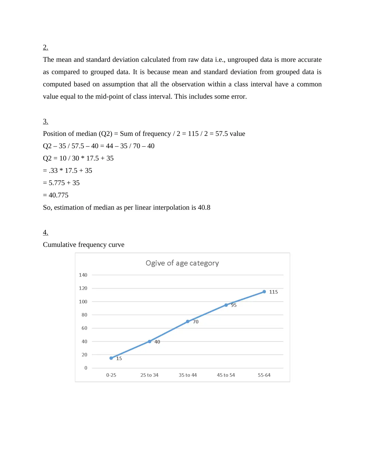
Position of median (Q2) = Sum of frequency / 2 = 115 / 2 = 57.5 value
Q2 – 35 / 57.5 – 40 = 44 – 35 / 70 – 40
Q2 = 10 / 30 * 17.5 + 35
= .33 * 17.5 + 35
= 5.775 + 35
= 40.775
So, estimation of median as per linear interpolation is 40.8
4.
Cumulative frequency curve

TASK 3
1.
Job
Separation*
(Probability
) Age
Gross
Hourly Pay
(£)
Commuting
Time
(Minutes)
Average
Weekly
Hours of
Work
Gender
(1 =
Male; 2 =
Female)
Job Separation*
(Probability) 1
Age
-
0.850933508 1
Gross Hourly
Pay (£)
-
0.780425444 0.526156257 1
Commuting
Time (Minutes) 0.862105058
-
0.782546734
-
0.682470154 1
Average Weekly
Hours of Work
-
0.180338317
-
0.029551426 0.377466662 0.017314834 1
Gender (1 =
Male; 2 =
Female) 0.225966998 0.007549337
-
0.419757353 0.004531325
-
0.964948544 1
Interpretation:
On the basis of above correlation matrix, the variable with highest correlation is consider as
best predictor. After analysing the above table, it is identified that the variable with highest
correlation is commuting time (minutes) and Job separation (probability) with the value of
0.8621 (Sun, Zhu and Zhou, 2020). Thus, the commuting time is a variable which is best
predictor as the relation between this two variable is highest amount the all other variable
correlation.

2.
3.
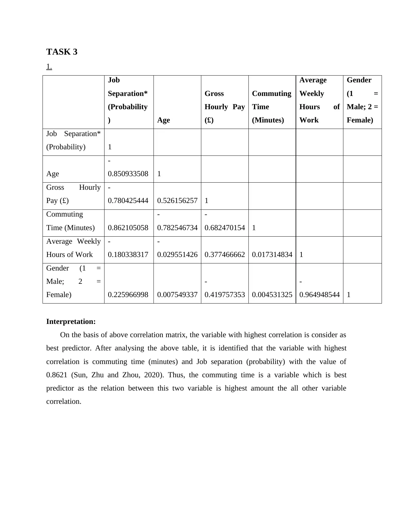
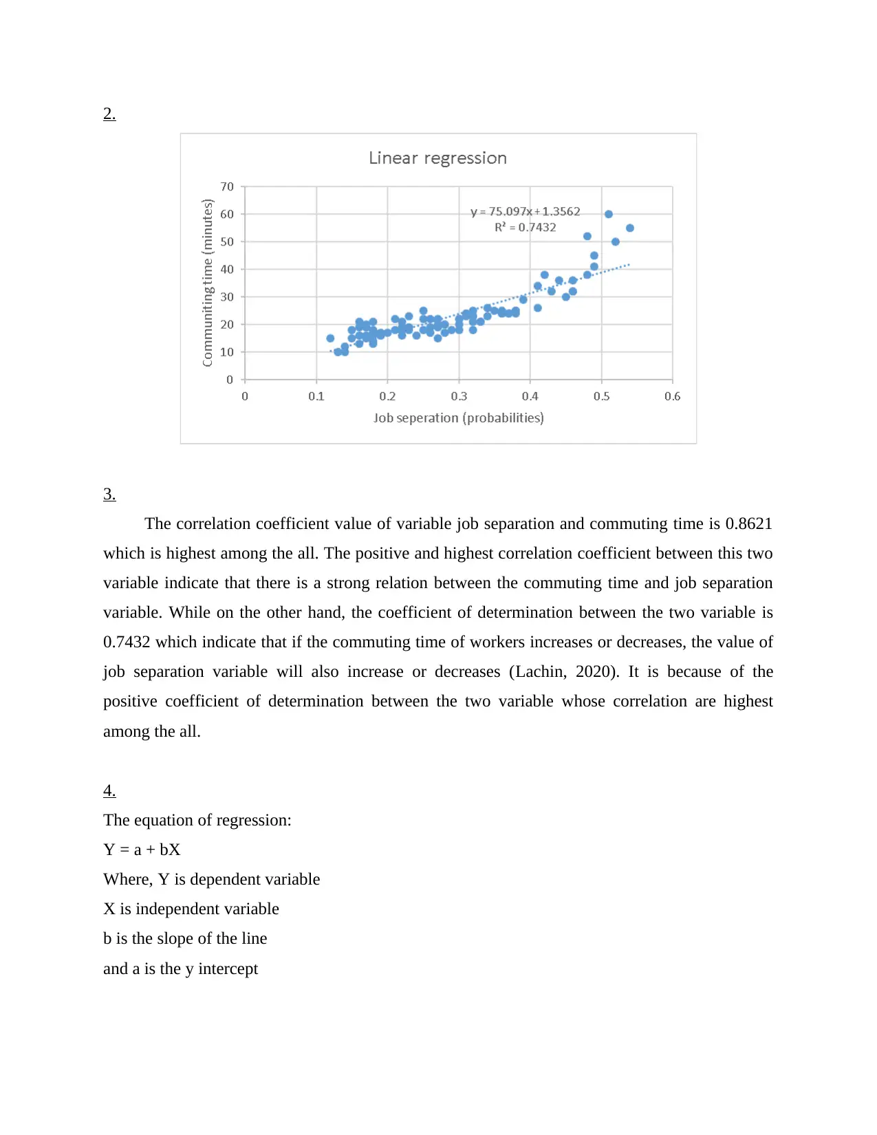
The correlation coefficient value of variable job separation and commuting time is 0.8621
which is highest among the all. The positive and highest correlation coefficient between this two
variable indicate that there is a strong relation between the commuting time and job separation
variable. While on the other hand, the coefficient of determination between the two variable is
0.7432 which indicate that if the commuting time of workers increases or decreases, the value of
job separation variable will also increase or decreases (Lachin, 2020). It is because of the
positive coefficient of determination between the two variable whose correlation are highest
among the all.
4.
The equation of regression:
Y = a + bX
Where, Y is dependent variable
X is independent variable
b is the slope of the line
and a is the y intercept

The regression equation of current variables is Y = 75.097x + 1.356 which state that there is a
positive relation between the dependent and independent variable. It means, with the change in
the commuting time variable (i.e., increase in the commuting time), the dependent variable such
as job separation will also change or increase (Marees and et.al., 2018).
TASK 4
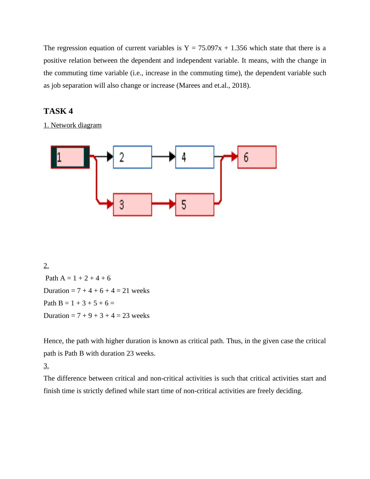
1. Network diagram
2.
Path A = 1 + 2 + 4 + 6
Duration = 7 + 4 + 6 + 4 = 21 weeks
Path B = 1 + 3 + 5 + 6 =
Duration = 7 + 9 + 3 + 4 = 23 weeks
Hence, the path with higher duration is known as critical path. Thus, in the given case the critical
path is Path B with duration 23 weeks.
3.
The difference between critical and non-critical activities is such that critical activities start and
finish time is strictly defined while start time of non-critical activities are freely deciding.

TASK 5
1.
I am able to perfectly create network diagram and identify critical path in this project. I also do
well in computing missing value of ungrouped descriptive statistics.
2.
I faced challenge in computing the mean and standard deviation of the grouped descriptive
statistics. It is because of my lack of attention during the learning session.
3.
When I will get the same project in future, I will use the excel function to make sure that my end
result of the data is right or wrong.

REFERENCES
Books and journals
Calle, M. L., 2019. Statistical analysis of metagenomics data. Genomics & informatics. 17(1).
Marees, A. T. and et.al., 2018. A tutorial on conducting genome‐wide association studies:
Quality control and statistical analysis. International journal of methods in psychiatric
research. 27(2). p.e1608.
Sun, S., Zhu, J. and Zhou, X., 2020. Statistical analysis of spatial expression patterns for spatially
resolved transcriptomic studies. Nature methods. 17(2). pp.193-200.
Lachin, J. M., 2020. Nonparametric statistical analysis. Jama. 323(20). pp.2080-2081.
Clifton, L. and Clifton, D. A., 2019. The correlation between baseline score and post-
intervention score, and its implications for statistical analysis. Trials. 20(1). pp.1-6.
1