OMGT2087: MOLP Model for Recycling Optimization Case Study

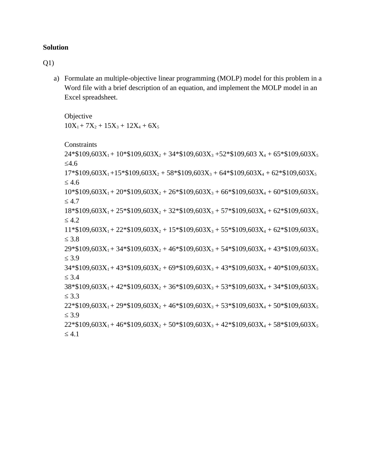
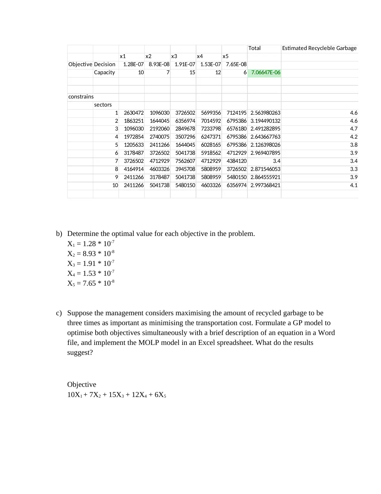
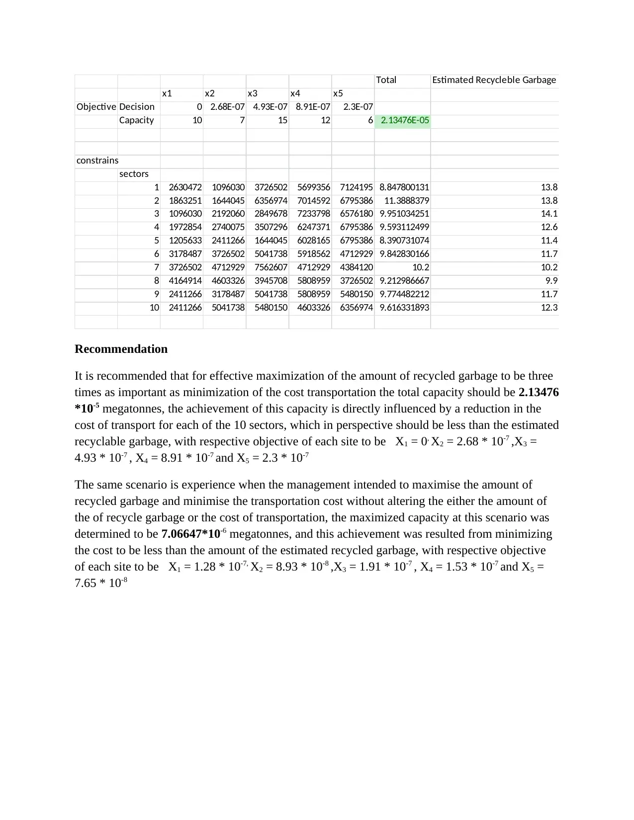
This assignment provides a comprehensive solution to a recycling optimization problem using a Multi-Objective Linear Programming (MOLP) model. The problem involves optimizing the collection and transportation of recyclable garbage from 10 sectors to five recycling sites, considering factors like recycling capacity, efficiency, and transportation costs. The solution includes the formulation of the MOLP model, its implementation in an Excel spreadsheet, and the determination of optimal values for each objective. Furthermore, it explores a goal programming (GP) model where maximizing recycled garbage is prioritized over minimizing transportation costs. The analysis offers recommendations based on the results of both models, suggesting optimal strategies for managing recyclable garbage effectively. Additionally, the assignment addresses warehouse location optimization using an NLP spreadsheet model and a van selection problem using a weighted scoring method, providing detailed steps and justifications for the recommendations. Finally, the selection of a location among three alternatives based on multiple criteria using a weighted normalized decision matrix is presented, ending with a final recommendation based on closeness to the ideal solution. The assignment uses quantitative methods to provide business insights and recommendations for complex decision-making scenarios.

Solution
Q1)
a) Formulate an multiple-objective linear programming (MOLP) model for this problem in a
Word file with a brief description of an equation, and implement the MOLP model in an
Excel spreadsheet.
Objective
10X1 + 7X2 + 15X3 + 12X4 + 6X5
Constraints
24*$109,603X1 + 10*$109,603X2 + 34*$109,603X3 +52*$109,603 X4 + 65*$109,603X5
≤4.6
17*$109,603X1 +15*$109,603X2 + 58*$109,603X3 + 64*$109,603X4 + 62*$109,603X5
≤ 4.6
10*$109,603X1 + 20*$109,603X2 + 26*$109,603X3 + 66*$109,603X4 + 60*$109,603X5
≤ 4.7
18*$109,603X1 + 25*$109,603X2 + 32*$109,603X3 + 57*$109,603X4 + 62*$109,603X5
≤ 4.2
11*$109,603X1 + 22*$109,603X2 + 15*$109,603X3 + 55*$109,603X4 + 62*$109,603X5
≤ 3.8
29*$109,603X1 + 34*$109,603X2 + 46*$109,603X3 + 54*$109,603X4 + 43*$109,603X5
≤ 3.9
34*$109,603X1 + 43*$109,603X2 + 69*$109,603X3 + 43*$109,603X4 + 40*$109,603X5
≤ 3.4
38*$109,603X1 + 42*$109,603X2 + 36*$109,603X3 + 53*$109,603X4 + 34*$109,603X5
≤ 3.3
22*$109,603X1 + 29*$109,603X2 + 46*$109,603X3 + 53*$109,603X4 + 50*$109,603X5
≤ 3.9
22*$109,603X1 + 46*$109,603X2 + 50*$109,603X3 + 42*$109,603X4 + 58*$109,603X5
≤ 4.1

Total Estimated Recycleble Garbage
x1 x2 x3 x4 x5
Objective Decision 1.28E-07 8.93E-08 1.91E-07 1.53E-07 7.65E-08
Capacity 10 7 15 12 6 7.06647E-06
constrains
sectors
1 2630472 1096030 3726502 5699356 7124195 2.563980263 4.6
2 1863251 1644045 6356974 7014592 6795386 3.194490132 4.6
3 1096030 2192060 2849678 7233798 6576180 2.491282895 4.7
4 1972854 2740075 3507296 6247371 6795386 2.643667763 4.2
5 1205633 2411266 1644045 6028165 6795386 2.126398026 3.8
6 3178487 3726502 5041738 5918562 4712929 2.969407895 3.9
7 3726502 4712929 7562607 4712929 4384120 3.4 3.4
8 4164914 4603326 3945708 5808959 3726502 2.871546053 3.3
9 2411266 3178487 5041738 5808959 5480150 2.864555921 3.9
10 2411266 5041738 5480150 4603326 6356974 2.997368421 4.1
b) Determine the optimal value for each objective in the problem.
X1 = 1.28 * 10-7
X2 = 8.93 * 10-8
X3 = 1.91 * 10-7
X4 = 1.53 * 10-7
X5 = 7.65 * 10-8
c) Suppose the management considers maximising the amount of recycled garbage to be
three times as important as minimising the transportation cost. Formulate a GP model to
optimise both objectives simultaneously with a brief description of an equation in a Word
file, and implement the MOLP model in an Excel spreadsheet. What do the results
suggest?
Objective
10X1 + 7X2 + 15X3 + 12X4 + 6X5

Constraints
24*$109,603X1 + 10*$109,603X2 + 34*$109,603X3 +52*$109,603 X4 + 65*$109,603X5
≤13.8
17*$109,603X1 +15*$109,603X2 + 58*$109,603X3 + 64*$109,603X4 + 62*$109,603X5
≤ 13.8
10*$109,603X1 + 20*$109,603X2 + 26*$109,603X3 + 66*$109,603X4 + 60*$109,603X5
≤ 14.1
18*$109,603X1 + 25*$109,603X2 + 32*$109,603X3 + 57*$109,603X4 + 62*$109,603X5
≤ 12.6
11*$109,603X1 + 22*$109,603X2 + 15*$109,603X3 + 55*$109,603X4 + 62*$109,603X5
≤ 11.4
29*$109,603X1 + 34*$109,603X2 + 46*$109,603X3 + 54*$109,603X4 + 43*$109,603X5
≤ 11.7
34*$109,603X1 + 43*$109,603X2 + 69*$109,603X3 + 43*$109,603X4 + 40*$109,603X5
≤ 10.2
38*$109,603X1 + 42*$109,603X2 + 36*$109,603X3 + 53*$109,603X4 + 34*$109,603X5
≤ 9.9
22*$109,603X1 + 29*$109,603X2 + 46*$109,603X3 + 53*$109,603X4 + 50*$109,603X5
≤ 11.7
22*$109,603X1 + 46*$109,603X2 + 50*$109,603X3 + 42*$109,603X4 + 58*$109,603X5
≤ 12.3

Total Estimated Recycleble Garbage
x1 x2 x3 x4 x5
Objective Decision 0 2.68E-07 4.93E-07 8.91E-07 2.3E-07
Capacity 10 7 15 12 6 2.13476E-05
constrains
sectors
1 2630472 1096030 3726502 5699356 7124195 8.847800131 13.8
2 1863251 1644045 6356974 7014592 6795386 11.3888379 13.8
3 1096030 2192060 2849678 7233798 6576180 9.951034251 14.1
4 1972854 2740075 3507296 6247371 6795386 9.593112499 12.6
5 1205633 2411266 1644045 6028165 6795386 8.390731074 11.4
6 3178487 3726502 5041738 5918562 4712929 9.842830166 11.7
7 3726502 4712929 7562607 4712929 4384120 10.2 10.2
8 4164914 4603326 3945708 5808959 3726502 9.212986667 9.9
9 2411266 3178487 5041738 5808959 5480150 9.774482212 11.7
10 2411266 5041738 5480150 4603326 6356974 9.616331893 12.3
Recommendation
It is recommended that for effective maximization of the amount of recycled garbage to be three
times as important as minimization of the cost transportation the total capacity should be 2.13476
*10-5 megatonnes, the achievement of this capacity is directly influenced by a reduction in the
cost of transport for each of the 10 sectors, which in perspective should be less than the estimated
recyclable garbage, with respective objective of each site to be X1 = 0, X2 = 2.68 * 10-7 ,X3 =
4.93 * 10-7 , X4 = 8.91 * 10-7 and X5 = 2.3 * 10-7
The same scenario is experience when the management intended to maximise the amount of
recycled garbage and minimise the transportation cost without altering the either the amount of
the of recycle garbage or the cost of transportation, the maximized capacity at this scenario was
determined to be 7.06647*10-6 megatonnes, and this achievement was resulted from minimizing
the cost to be less than the amount of the estimated recycled garbage, with respective objective
of each site to be X1 = 1.28 * 10-7, X2 = 8.93 * 10-8 ,X3 = 1.91 * 10-7 , X4 = 1.53 * 10-7 and X5 =
7.65 * 10-8

Q2)
The NLP spreadsheet model is following:
Formulas:
G2 =D2*((B2-$B$23)^2+(C2-$C$23)^2)^0.5+E2*((B2-$B$24)^2+(C2-
$C$24)^2)^0.5+F2*((B2-$B$25)^2+(C2-$C$25)^2)^0.5 copy to G2:G21
H2 =SUM(D2:F2) copy to H2:H21
G23 =SUM(G2:G21)
The locations of the three warehouses are following
X Y
Wh 1: 13.1 10.4
Wh 2: 23.9 10.8
Wh 3: 5.0 4.6
The subrubs are supplied by the warehouses as indicated in the matrix (D2:F21). Value 1
indicates that particular Suburb is supplied by that warehouse.

Recommendation
It is recommended that for a company to build its warehouses in locations that minimise the
distances to each of the stations it serves, the location of the three warehouse from the suburbs X
and Y for warehouse 1 should be 13.1 and 10.4, similarly warehouse 2 should be 23.9 and 10.8
and finally the warehouse 3 location should be 5.0 and 4.6 respectively, therefore to determine
the respective distance from the respective petrol station there location will be based on the
respective reference for of the position of the three warehouse which will result to a total
distance which is equal 86, this is the best minimum total distance from all the station that
should be considered as far as the position of the warehouse is concern

Q3)
Step 1. Determine the priority of the factors which are taken into the consideration. The factors
taken into consideration for the van here are – price, safety, economy, and comfort.
How to find the priority-
1. Find the geometric mean of all the factors, of their rank factors. GM = (factor 1*factor
2*..factor n)1/n
2. Find the priority vector for each factor, priority vector = GM of the factor/ (Sum of all
GMs). This gives the actual priority values of all the factors. But now we also need to
check the consistency of the data, consistency means that the data is valid to use, for this
we need to find the Consistency Ratio
3. Finding the CR- Find the sum of all columns as below-

4. Now we multiply the sum of columns of the factors into their respective PVs. See below
5. Now we find the sum of all the Sum PV values, this sum will be the value called lambda
max
6. Now we find Consistency Index; CI; CI= (lamda max- n)/(n-1); n= number of factors; 4
here. As shown below. CI=0.024

7. There is a term random index (RI) corresponding to number of fators; for n=4; RI=0.9.
CR=CI/RI/ See below. If CR is below 0.1; then data is consistent and can be used. The
CR value is .0264; hence the data is consistent
8. Now, we find the same CR for all the other 4 matrices; that is Van A,B,C against Price,
safety, economy and comfort. Find the PVs of all the Vans against all the factors, using
the same procedure described above. Check their consistency at all levels. Use RI for n=3
as 0.58. As shown below

You see that for comfort and economy, the CR is above 0.1; hence the data is inconsistent and
should be disregarded, but here we can continue to solve the question.

Now we make the final matrix, to find the final rank. For all the Van, A,B,C, write their PV
values against the corresponding 4 factors; which we found above. Also write the PV values
we found of the four factors.
Now, multiply the PV of the factor, to the corresponding PV of the respective Van, and find
the final score of each van. For eg; for Van A; score = D40*D39 + E40*E39 + F40*F39 +
G40*G39; and do so for all the Vans. See below