Water Supply Network Distribution and Clean Sewer System Design
VerifiedAdded on 2023/06/08
|24
|3532
|220
Report
AI Summary
This report presents an analysis and design survey for water supply network distribution and sewer systems, focusing on the design methodology for clean sewer frameworks considering pseudo-plastic fluid conditions when effluent mixes with water. It details the design of a pipeline circulation network, outlining assumptions related to particles, temperature, speed, and other critical properties influencing water and sewer characteristics. The report discusses the Hardy Cross method for analyzing pipe networks, emphasizing its approach to nonlinear conditions and potential modifications for enhanced convergence. Specific objectives include determining nodal heads, pipe discharges, nodal inflows/outflows, and pipe resistance constants. The methodology involves dividing the network into loops, making flow assumptions, calculating equivalent resistance, and iteratively correcting flows until head loss changes become minimal, ultimately solving for total pressure at each node using the energy method.

Abstract
This report shows and surveys the extent of possible design for the water supply network
distribution and the design for sewer system. This report begins with the analysis of water supply
network distribution. The design methodology in this report for clean sewer framework will be
actualized in perspective of the conditions of pseudo-plastic fluids. At the point when profluent
is mixed with water, it acts as pseudo-plastic. This report shows the design of pipeline circulation
network. Assumption has been considered on the particles, temperature and speed and other
basic properties that may impact the water and sewer properties
Paraphrase This Document
Need a fresh take? Get an instant paraphrase of this document with our AI Paraphraser

Introduction
The pipe network system for series and parallel each do have a point when the flows enters the
system and on the other point where the flow is exiting, permitting the flow course in each and
every pipe to be derived explicitly. For such a case, in the event that we are simply intrigued by
the connection between total flow and aggregate head loss, it is some of the time helpful to
improve the analysis by representation of the entire group of pipes as a solitary, using hydraulic
water identical pipe.
The piping system for the friction intensity constraint for every pipe should always be known,
and it should be free of the flow situations for the scope of flow states of intrigue. In the event
that the distribution water condition is utilized to relate head loss hL to velocity V or flow rate Q
(Spiliotis and Tsakiris, 2010), the representation of friction intensity factor is denoted by f, this
has a steady value on a specific pipe for completely turbulent flow, however it does not imply on
the transitional or laminar flow. In the event that the Hazen Williams equation (Kumar,
Narasimhan and Bhallamudi, 2010) is utilized, the friction intensity factor is CHW, which is
thought to be identified for a specific pipe.
The Hardy cross method used in analyzing the pipe network system illuminate the nonlinear
conditions associated with network investigation by making certain assumptions. The higher
power rectification terms can be dismissed and the loop number is little for a solitary loop
despite the fact that the underlying guess is weak. However, dismissing contiguous loops and
considering just a single amendment condition at once can influence the arrangement and
furthermore number of iteration required for joining increments as the measure of the system
increments.
Altered Hardy Cross strategy can be connected to enhance merging and lessen the quantity of
loops. In any case, this number can be very substantial for genuine systems. Consequently, rather
than considering just a single amendment condition at once, all the adjustment conditions can be
illuminated by thinking about the impact of every single contiguous circle. So joining can be
accomplished in fewer loops. Additionally, a portion of the conditions engaged with pipe
network investigation is nonlinear.

Since there is no immediate technique for their answer, these conditions are linearized and after
that tackled.
Since the arrangement is estimated, it is remedied and the iterative method is proceeded until the
point when attractive precision is come to. The Newton-Raphson strategy and the Linear Theory
technique endeavor to comprehend all the concerned conditions all the while by applying the
iterative methodology.
The Newton-Raphson strategy (Kulworawanichpong., 2010) extends the nonlinear terms in
Taylor– s arrangement, considers just the direct terms by dismissing the deposits after two terms.
Since the nonlinearity in the conditions for pipe organize examination is uniform and basic , the
nonlinear term can be effectively linearized by consolidating a piece of the nonlinear term into
the pipe opposition consistent. This standard was first utilized by McIlroy Then, Wood and
Charles] created it and it is presently generally utilized as a part of training. This standard can be
utilized to linearize a wide range of conditions. Nonetheless, by and by it is connected to pipe-
release conditions and nodal-head conditions.
A node with a known head is generally a source hub, for example, a hoisted stockpiling tank. A
node with a known stream is a request node
•At the source node, the flow is for the most part unknown,
•While at the request node, the head is for the most part obscure.
Be that as it may, sometimes the stream additionally might be known notwithstanding the known
head at a source hub, while the stream may likewise be obscure notwithstanding the obscure
head at a request hub.
Specific objectives
1. To determine nodal heads, H
2. To determine pipe discharges, Q
3. To determine nodal inflows or outflows, q
4. To determine pipe resistance constants, R
⊘ This is a preview!⊘
Do you want full access?
Subscribe today to unlock all pages.

Trusted by 1+ million students worldwide

Considering a network that has different loops, at normal circumstances there will be channels
regular to bordering loops with a clockwise stream in one loop showing up a countercurrent flow
to clockwise in the other. Each loop must be distinguished and the rectifications made efficiently
to each loop thus. The remedy to the flows must be made each time before proceeding onward to
the following loop. In the excess of two loops in a system, the procedure turns out to be
extremely intricate and computer strategies should be utilized.
Paraphrase This Document
Need a fresh take? Get an instant paraphrase of this document with our AI Paraphraser
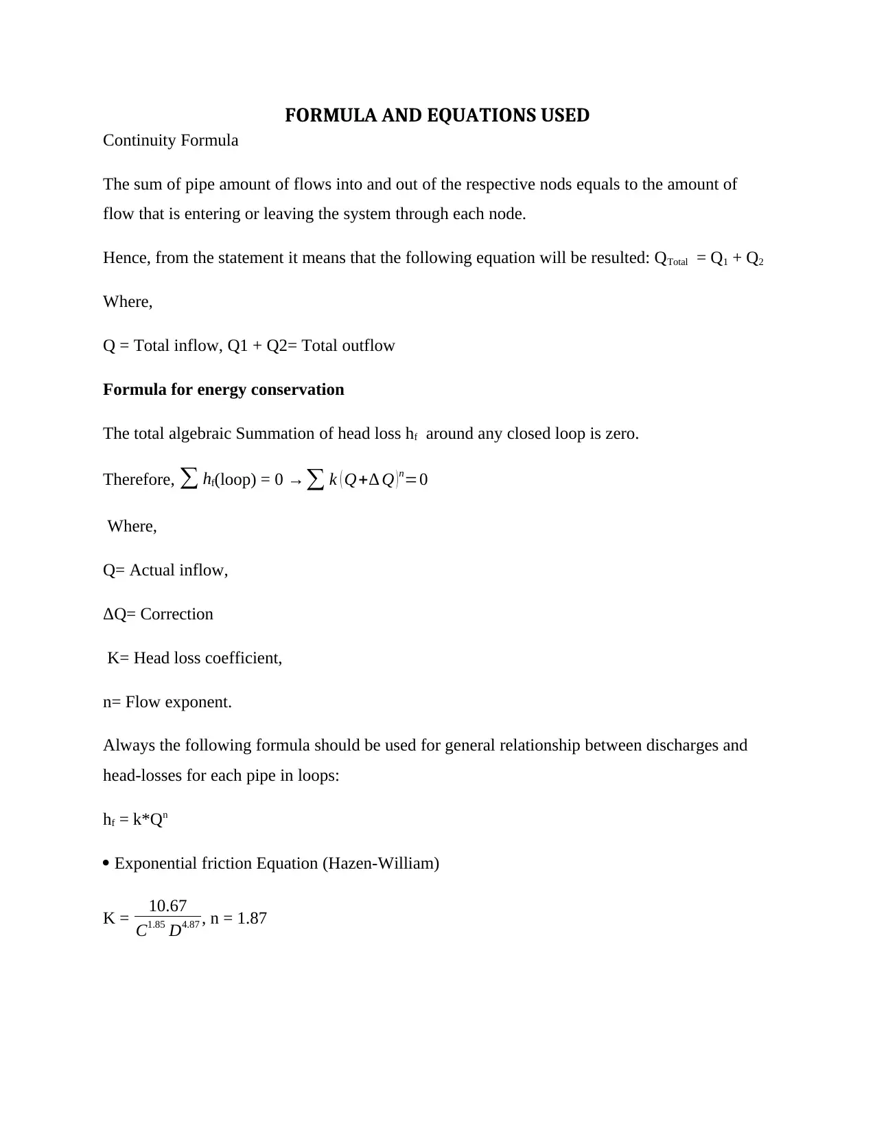
FORMULA AND EQUATIONS USED
Continuity Formula
The sum of pipe amount of flows into and out of the respective nods equals to the amount of
flow that is entering or leaving the system through each node.
Hence, from the statement it means that the following equation will be resulted: QTotal = Q1 + Q2
Where,
Q = Total inflow, Q1 + Q2= Total outflow
Formula for energy conservation
The total algebraic Summation of head loss hf around any closed loop is zero.
Therefore, ∑ hf(loop) = 0 →∑ k ( Q+∆ Q )n=0
Where,
Q= Actual inflow,
ΔQ= Correction
K= Head loss coefficient,
n= Flow exponent.
Always the following formula should be used for general relationship between discharges and
head-losses for each pipe in loops:
hf = k*Qn
Exponential friction Equation (Hazen-William)
K = 10.67
C1.85 D4.87 , n = 1.87

∆ Q= −∑ h
2∗∑( h
Q )
Methodology
With respect to pipe network investigation, the conventionally approach is known as the Hardy
Cross procedure (Huang, Vairavamoorthy and Tsegaye, 2010). This strategy is appropriate if the
entire pipe sizes (lengths and breadths) are settled, and either the head losses between the outlets
and inlets are known yet the flow are not, or the flow at each inflow and overflowing point are
known, yet the head losses are definitely not. This last case is investigated straightaway.
The system incorporates making a guess with respect to the flow to rate in each pipe, taking
consideration of making a guess to such an extent that the total flow into any crossing point
approaches the total flow out of that convergence. By then the head loss in each pipe is found
out, in perspective of the normal flow and the picked flow versus head loss relationship. Next,
the system is checked whether the head loss around each loop is zero. Since the fundamental
flow was speculated, this will undoubtedly not be the circumstance. The flow rates are then
adjusted with the end goal that continuity will in any case be fulfilled at each crossing point,
aside from the head loss around each loop is more similar to be zero. This strategy is repeated
until the point that the progressions are attractively little. The definite procedure is according to
the following
Procedure
Divided the network into loops
For each loops done the fallowing steps
1. Assumptions on the flow, , flow course in the pipes, direction of flow in the loop where
positive will be taken to be clockwise or negative will be taken to be counterclockwise,
with an application of equation of continuity condition at every node. Evaluated pipe
flows are associated with iteration until head loss in the clockwise direction is equivalent
to the counterclockwise bearing in each loop.
⊘ This is a preview!⊘
Do you want full access?
Subscribe today to unlock all pages.

Trusted by 1+ million students worldwide
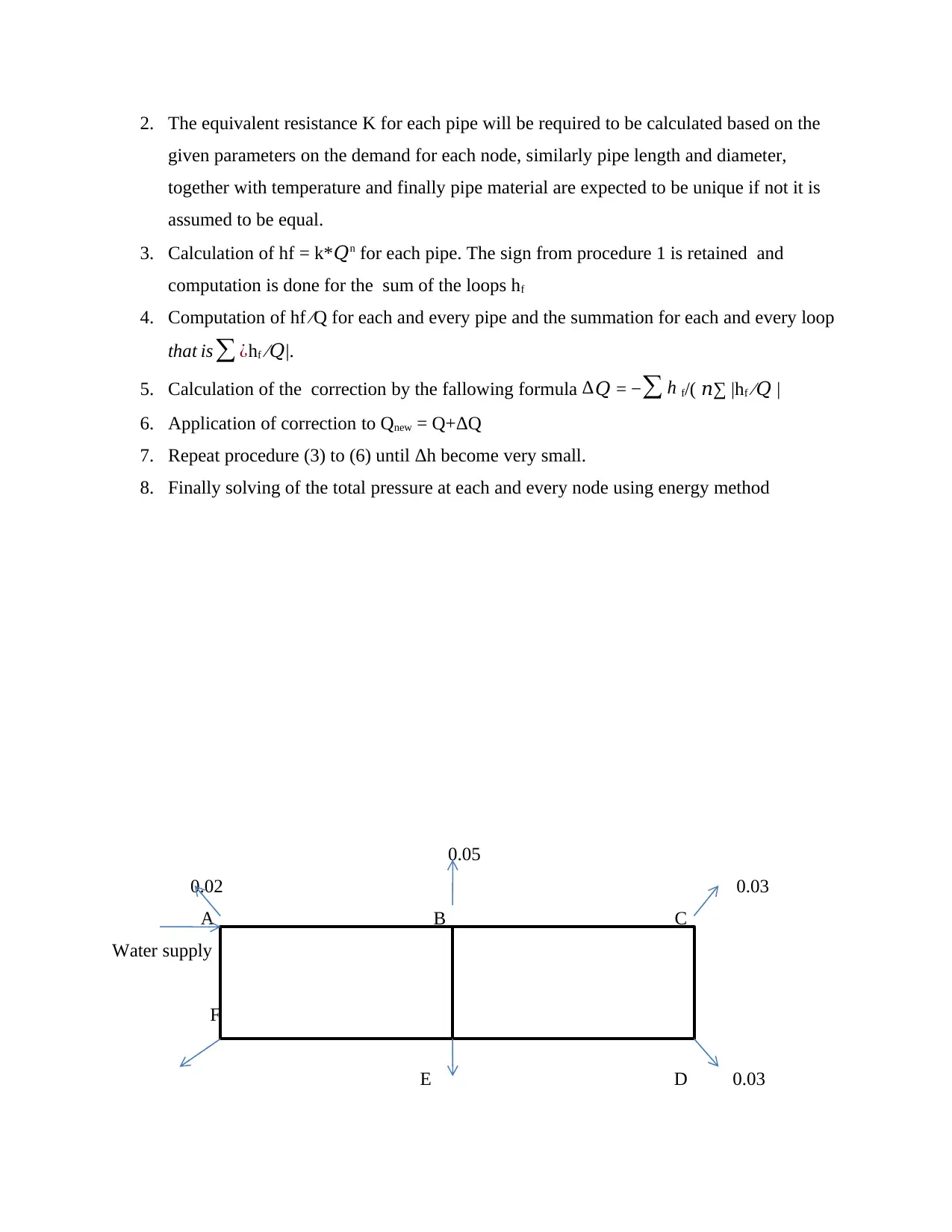
2. The equivalent resistance K for each pipe will be required to be calculated based on the
given parameters on the demand for each node, similarly pipe length and diameter,
together with temperature and finally pipe material are expected to be unique if not it is
assumed to be equal.
3. Calculation of hf = k*𝑄n for each pipe. The sign from procedure 1 is retained and
computation is done for the sum of the loops hf
4. Computation of hf ⁄Q for each and every pipe and the summation for each and every loop
that is∑ ¿hf ⁄𝑄|.
5. Calculation of the correction by the fallowing formula ∆𝑄 = − ∑ h f/( 𝑛∑ |hf ⁄𝑄 |
6. Application of correction to Qnew = Q+ΔQ
7. Repeat procedure (3) to (6) until Δh become very small.
8. Finally solving of the total pressure at each and every node using energy method
0.05
0.02 0.03
A B C
Water supply
F
E D 0.03
Paraphrase This Document
Need a fresh take? Get an instant paraphrase of this document with our AI Paraphraser
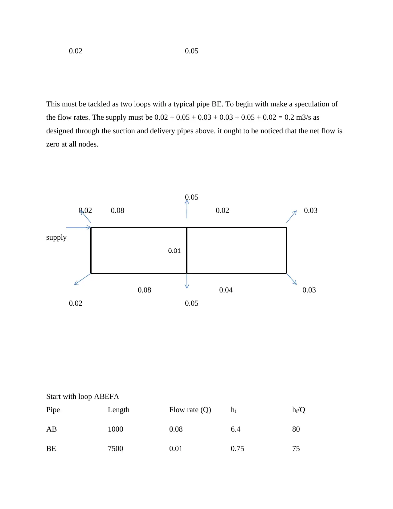
0.02 0.05
This must be tackled as two loops with a typical pipe BE. To begin with make a speculation of
the flow rates. The supply must be 0.02 + 0.05 + 0.03 + 0.03 + 0.05 + 0.02 = 0.2 m3/s as
designed through the suction and delivery pipes above. it ought to be noticed that the net flow is
zero at all nodes.
0.05
0.02 0.08 0.02 0.03
supply
0.08 0.04 0.03
0.02 0.05
Start with loop ABEFA
Pipe Length Flow rate (Q) hf hf/Q
AB 1000 0.08 6.4 80
BE 7500 0.01 0.75 75
0.01
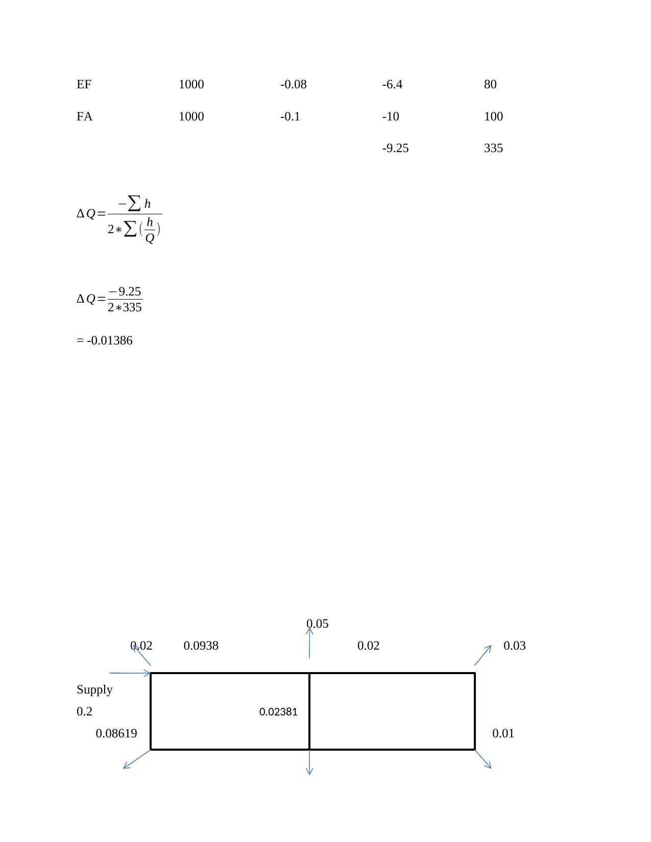
EF 1000 -0.08 -6.4 80
FA 1000 -0.1 -10 100
-9.25 335
∆ Q= −∑ h
2∗∑( h
Q )
∆ Q=−9.25
2∗335
= -0.01386
0.05
0.02 0.0938 0.02 0.03
Supply
0.2
0.08619 0.01
0.02381
FA 1000 -0.1 -10 100
-9.25 335
∆ Q= −∑ h
2∗∑( h
Q )
∆ Q=−9.25
2∗335
= -0.01386
0.05
0.02 0.0938 0.02 0.03
Supply
0.2
0.08619 0.01
0.02381
⊘ This is a preview!⊘
Do you want full access?
Subscribe today to unlock all pages.

Trusted by 1+ million students worldwide
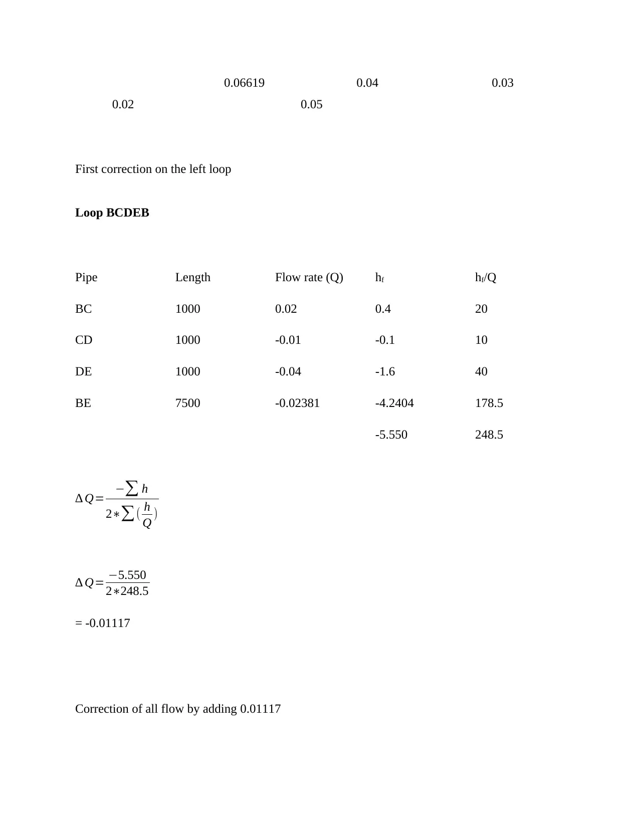
0.06619 0.04 0.03
0.02 0.05
First correction on the left loop
Loop BCDEB
Pipe Length Flow rate (Q) hf hf/Q
BC 1000 0.02 0.4 20
CD 1000 -0.01 -0.1 10
DE 1000 -0.04 -1.6 40
BE 7500 -0.02381 -4.2404 178.5
-5.550 248.5
∆ Q= −∑ h
2∗∑( h
Q )
∆ Q= −5.550
2∗248.5
= -0.01117
Correction of all flow by adding 0.01117
0.02 0.05
First correction on the left loop
Loop BCDEB
Pipe Length Flow rate (Q) hf hf/Q
BC 1000 0.02 0.4 20
CD 1000 -0.01 -0.1 10
DE 1000 -0.04 -1.6 40
BE 7500 -0.02381 -4.2404 178.5
-5.550 248.5
∆ Q= −∑ h
2∗∑( h
Q )
∆ Q= −5.550
2∗248.5
= -0.01117
Correction of all flow by adding 0.01117
Paraphrase This Document
Need a fresh take? Get an instant paraphrase of this document with our AI Paraphraser
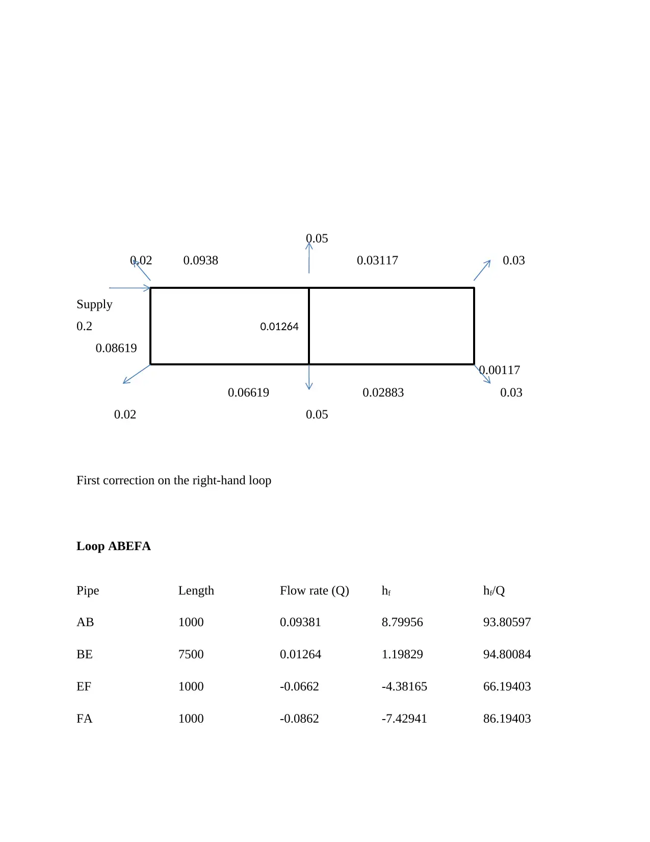
0.05
0.02 0.0938 0.03117 0.03
Supply
0.2
0.08619
0.00117
0.06619 0.02883 0.03
0.02 0.05
First correction on the right-hand loop
Loop ABEFA
Pipe Length Flow rate (Q) hf hf/Q
AB 1000 0.09381 8.79956 93.80597
BE 7500 0.01264 1.19829 94.80084
EF 1000 -0.0662 -4.38165 66.19403
FA 1000 -0.0862 -7.42941 86.19403
0.01264
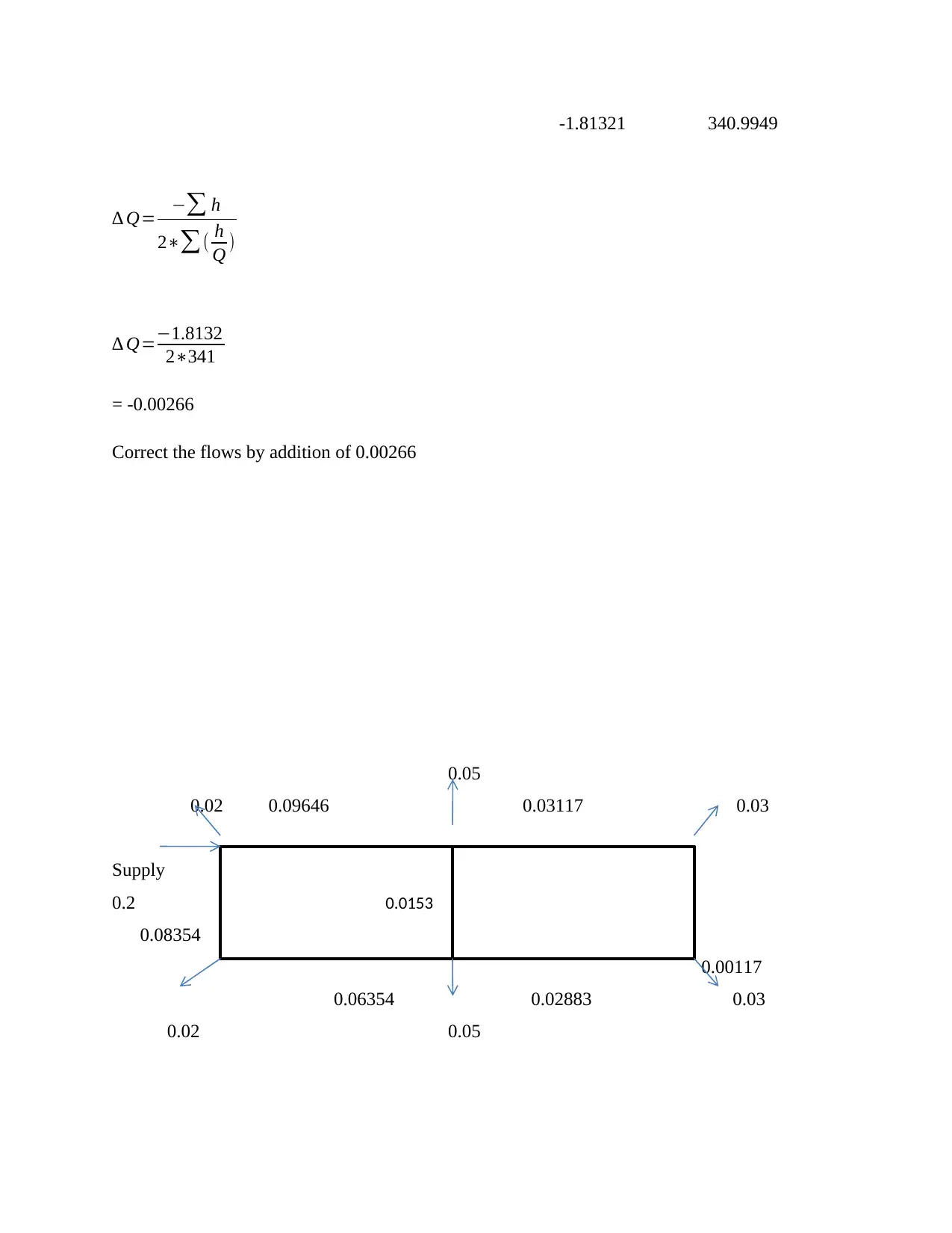
-1.81321 340.9949
∆ Q= −∑ h
2∗∑( h
Q )
∆ Q=−1.8132
2∗341
= -0.00266
Correct the flows by addition of 0.00266
0.05
0.02 0.09646 0.03117 0.03
Supply
0.2
0.08354
0.00117
0.06354 0.02883 0.03
0.02 0.05
0.0153
∆ Q= −∑ h
2∗∑( h
Q )
∆ Q=−1.8132
2∗341
= -0.00266
Correct the flows by addition of 0.00266
0.05
0.02 0.09646 0.03117 0.03
Supply
0.2
0.08354
0.00117
0.06354 0.02883 0.03
0.02 0.05
0.0153
⊘ This is a preview!⊘
Do you want full access?
Subscribe today to unlock all pages.

Trusted by 1+ million students worldwide
1 out of 24
Your All-in-One AI-Powered Toolkit for Academic Success.
+13062052269
info@desklib.com
Available 24*7 on WhatsApp / Email
![[object Object]](/_next/static/media/star-bottom.7253800d.svg)
Unlock your academic potential
Copyright © 2020–2026 A2Z Services. All Rights Reserved. Developed and managed by ZUCOL.


