World Health and Population Analysis

World Health and Population Analysis 1
WORLD HEALTH AND POPULATION ANALYSIS
Name
Course Number
Date
Faculty Name

World Health and Population Analysis 2
World Health and Population Analysis
1. Introduction
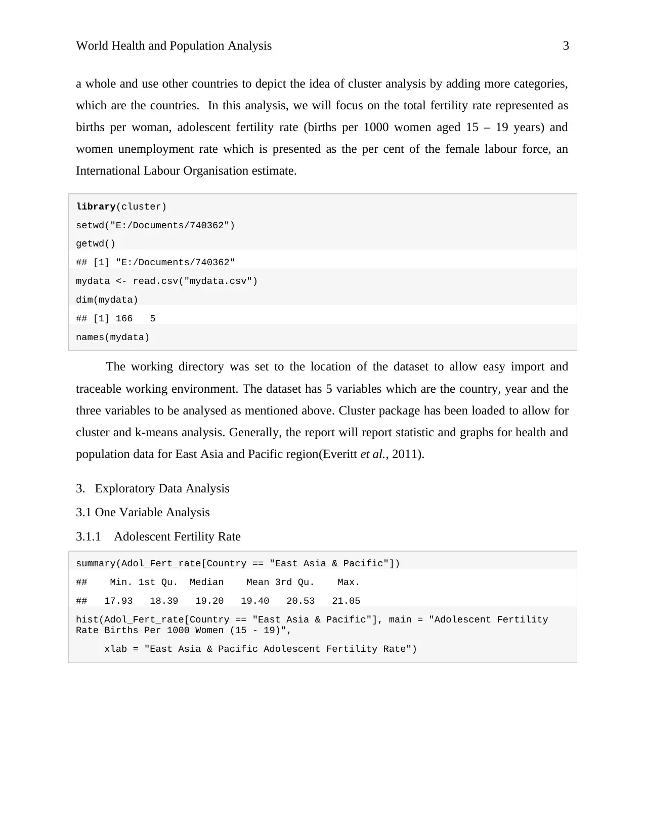
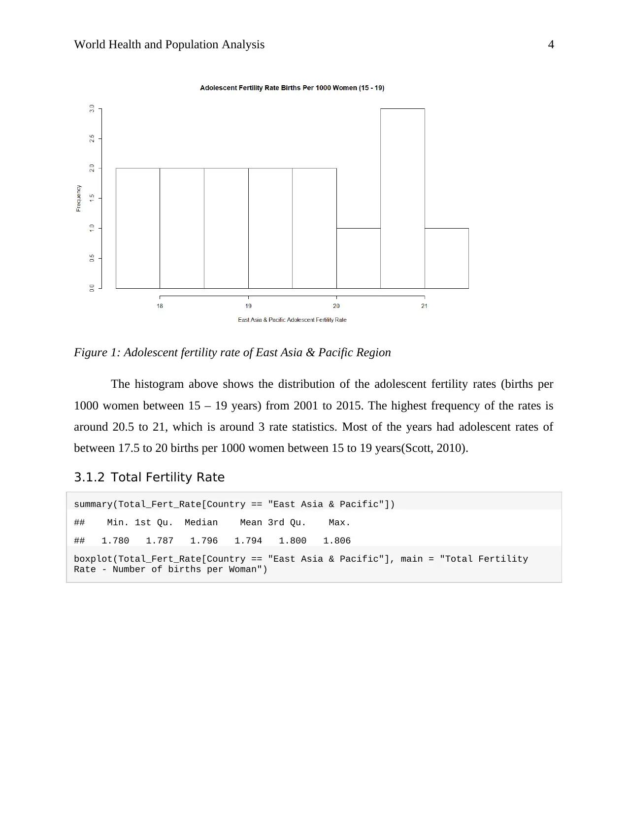
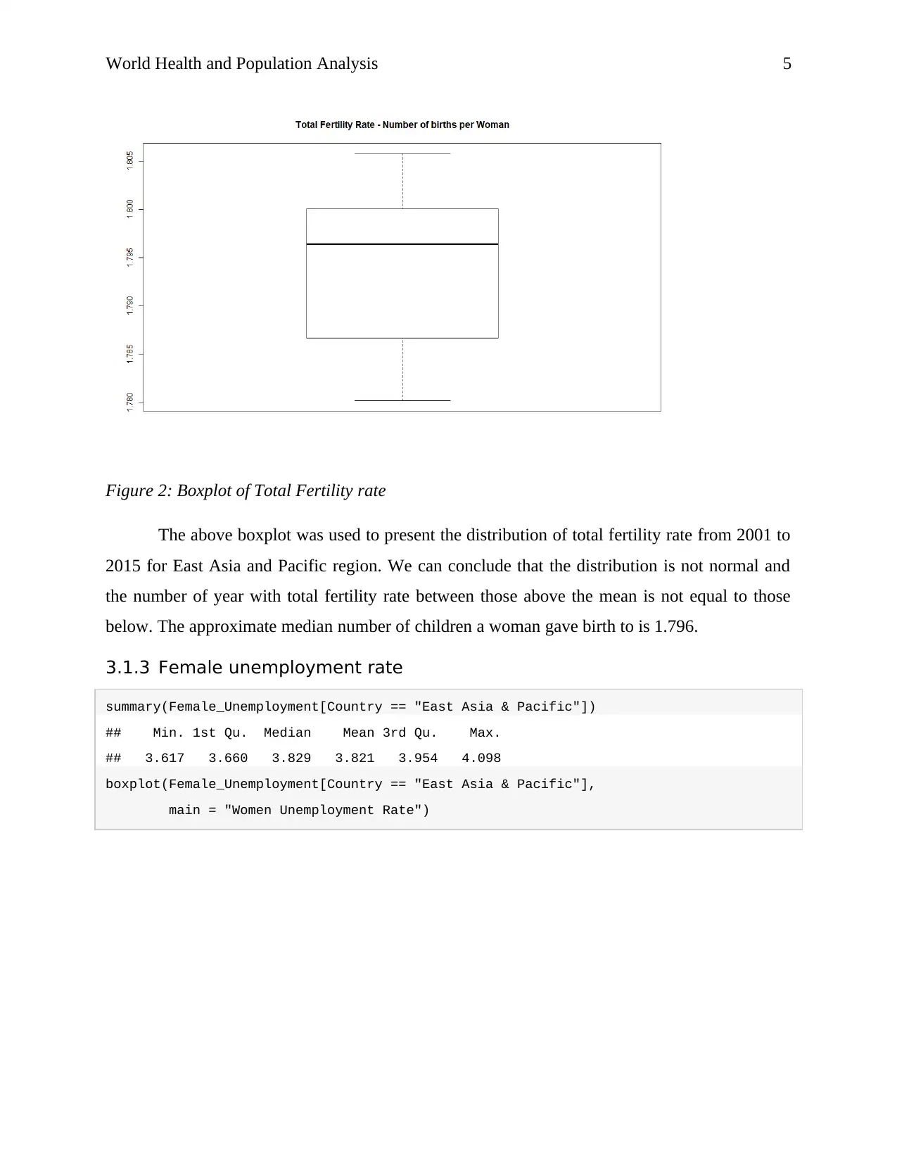
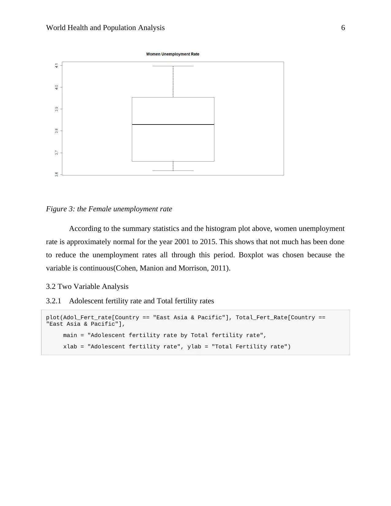
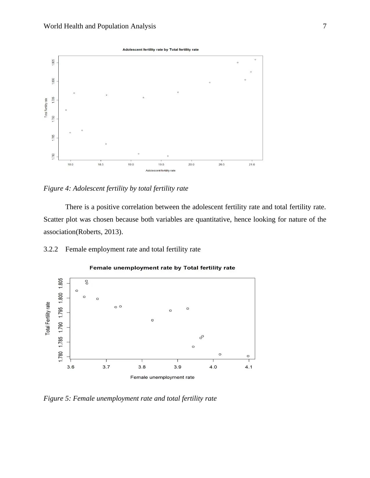
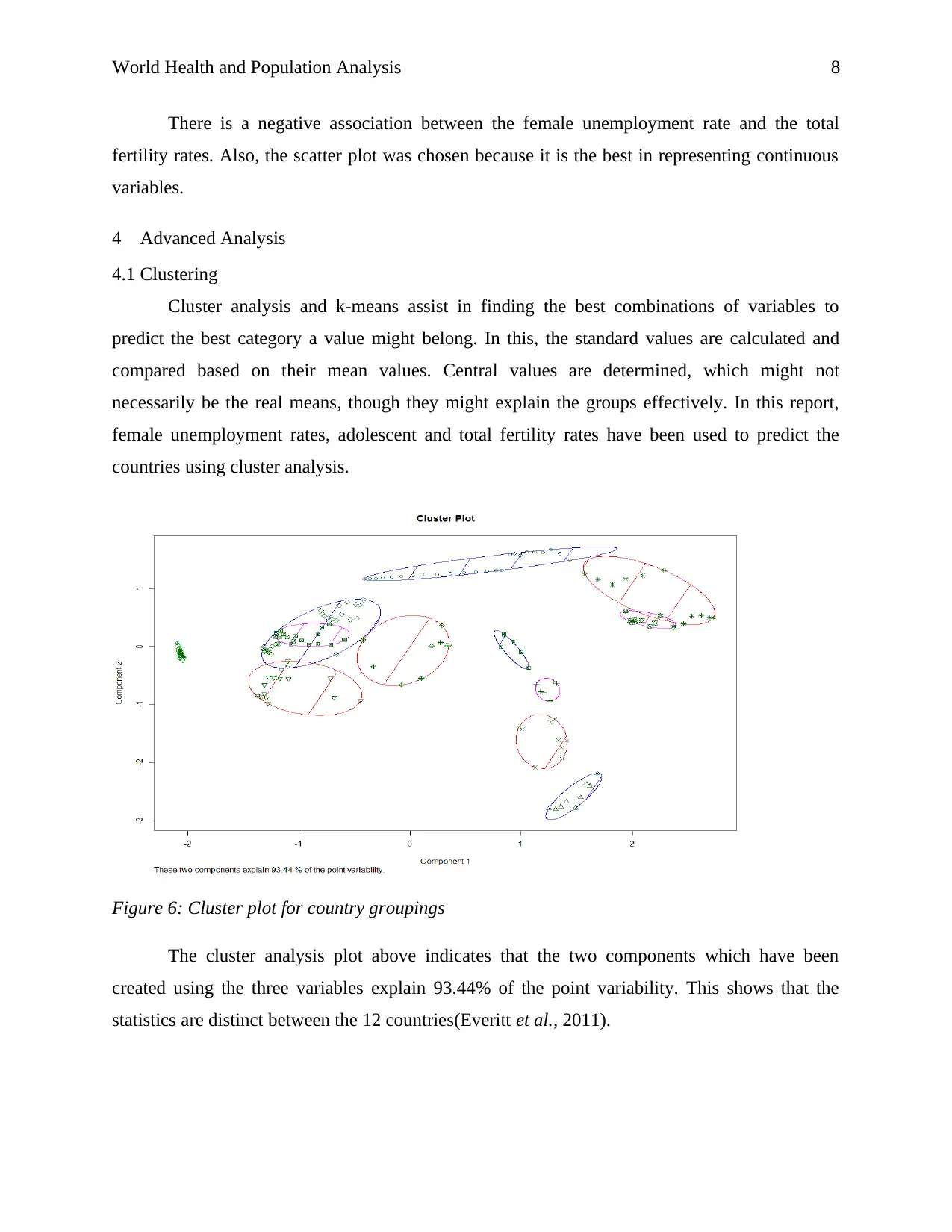
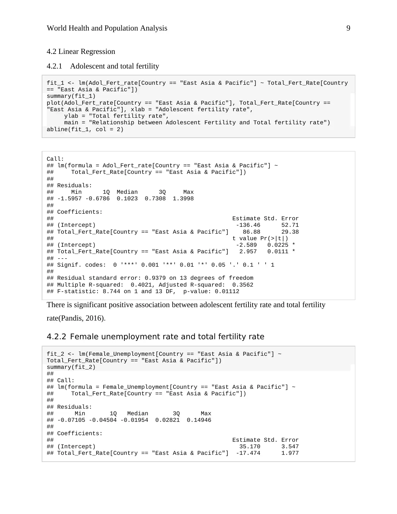
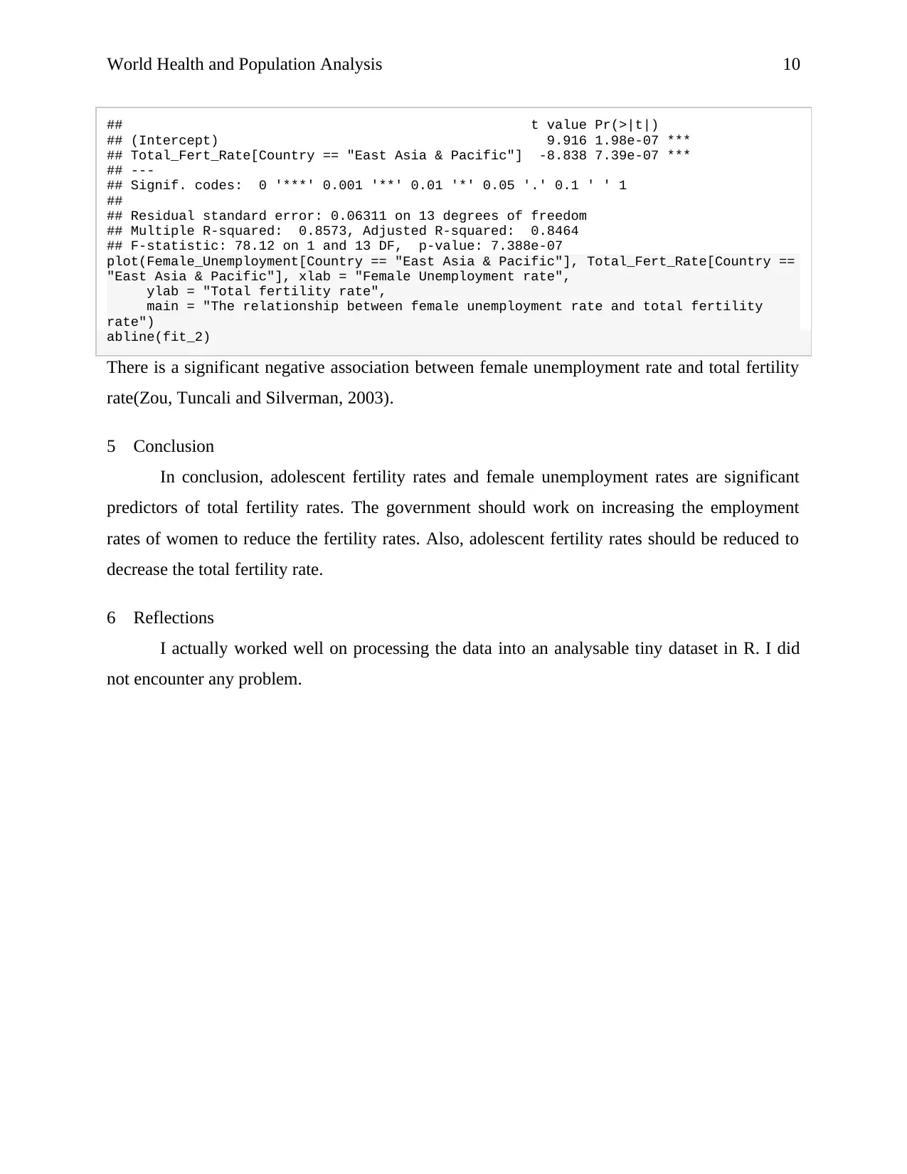
In this data analysis, health and population statistics will be presented for East Asian and
Pacific countries. It is an open report without fixed objectives but in this paper will focus on
health issues and factors that might affect the total fertility of a woman from 2001 to 2015. The
development of a country is determined by various factors which should be improved as a whole.
As a result, countries are making policies which are focused on the general development as
opposed to dedicated approaches. Further, research has also taken an important role in
supporting the informed decision to the government and non-governmental organisations. The
target group for this report is the government agencies, researchers and business legislatures.
The main limitation of this report is that it only includes information from East Asia and
Pacific region information, hence it may not be generalizable to other areas across the world.
Also, it might not feasible to countercheck the validity of the data because we only depend on
data from the World Bank. The data will be downloaded from the World Bank development
indicators database, extracted and filtered using the MS Excel software to fit the criteria of this
report. Using the advanced filter of MS Excel, the selected filter names for this report will be
used to select the rows which include such data for analysis. Also, data from 2001 to 2015 will
be extracted because this report as stated in the assignment requirements.
One variable, two variable, cluster and linear regression statistical techniques will use
present and extract information from the data. For the one and two analysis, appropriate graphs
will be used to present the data and explanations provided about the distributions and
relationships. Further, cluster analysis and k-means techniques will be briefly explained. The
cluster analysis will be performed to understand explain some groupings. Lastly, simple linear
regression technique to explain some relationships between variables – with linear plots created
to depict their correlation.
2. Data Setup
Data pre-processing is required to create a tidy dataset which is analysable using the r
software. First, it will be important to understand the variables to be analysed – which will guide
the analysis stage. This will allow a focused analysis for the East Asia and Pacific region data as

World Health and Population Analysis 3
a whole and use other countries to depict the idea of cluster analysis by adding more categories,
which are the countries. In this analysis, we will focus on the total fertility rate represented as
births per woman, adolescent fertility rate (births per 1000 women aged 15 – 19 years) and
women unemployment rate which is presented as the per cent of the female labour force, an
International Labour Organisation estimate.
library(cluster)
setwd("E:/Documents/740362")
getwd()
## [1] "E:/Documents/740362"
mydata <- read.csv("mydata.csv")
dim(mydata)
## [1] 166 5
names(mydata)
The working directory was set to the location of the dataset to allow easy import and
traceable working environment. The dataset has 5 variables which are the country, year and the
three variables to be analysed as mentioned above. Cluster package has been loaded to allow for
cluster and k-means analysis. Generally, the report will report statistic and graphs for health and
population data for East Asia and Pacific region(Everitt et al., 2011).
3. Exploratory Data Analysis
3.1 One Variable Analysis
3.1.1 Adolescent Fertility Rate
summary(Adol_Fert_rate[Country == "East Asia & Pacific"])
## Min. 1st Qu. Median Mean 3rd Qu. Max.
## 17.93 18.39 19.20 19.40 20.53 21.05
hist(Adol_Fert_rate[Country == "East Asia & Pacific"], main = "Adolescent Fertility
Rate Births Per 1000 Women (15 - 19)",
xlab = "East Asia & Pacific Adolescent Fertility Rate")

World Health and Population Analysis 4
Figure 1: Adolescent fertility rate of East Asia & Pacific Region
The histogram above shows the distribution of the adolescent fertility rates (births per
1000 women between 15 – 19 years) from 2001 to 2015. The highest frequency of the rates is
around 20.5 to 21, which is around 3 rate statistics. Most of the years had adolescent rates of
between 17.5 to 20 births per 1000 women between 15 to 19 years(Scott, 2010).
3.1.2 Total Fertility Rate
summary(Total_Fert_Rate[Country == "East Asia & Pacific"])
## Min. 1st Qu. Median Mean 3rd Qu. Max.
## 1.780 1.787 1.796 1.794 1.800 1.806
boxplot(Total_Fert_Rate[Country == "East Asia & Pacific"], main = "Total Fertility
Rate - Number of births per Woman")