Factors Influencing Academic Performance: BSB123 Data Analysis Report

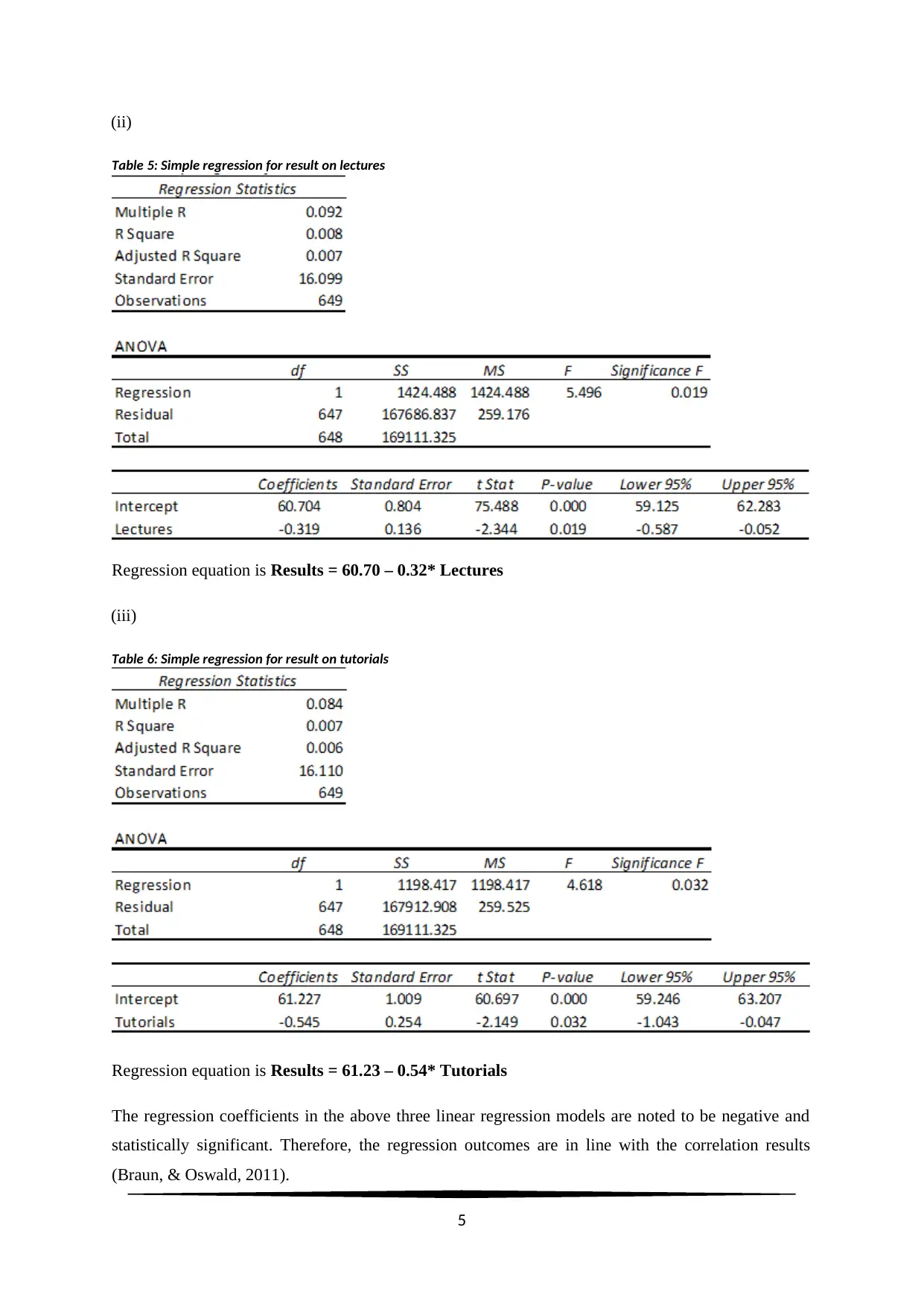
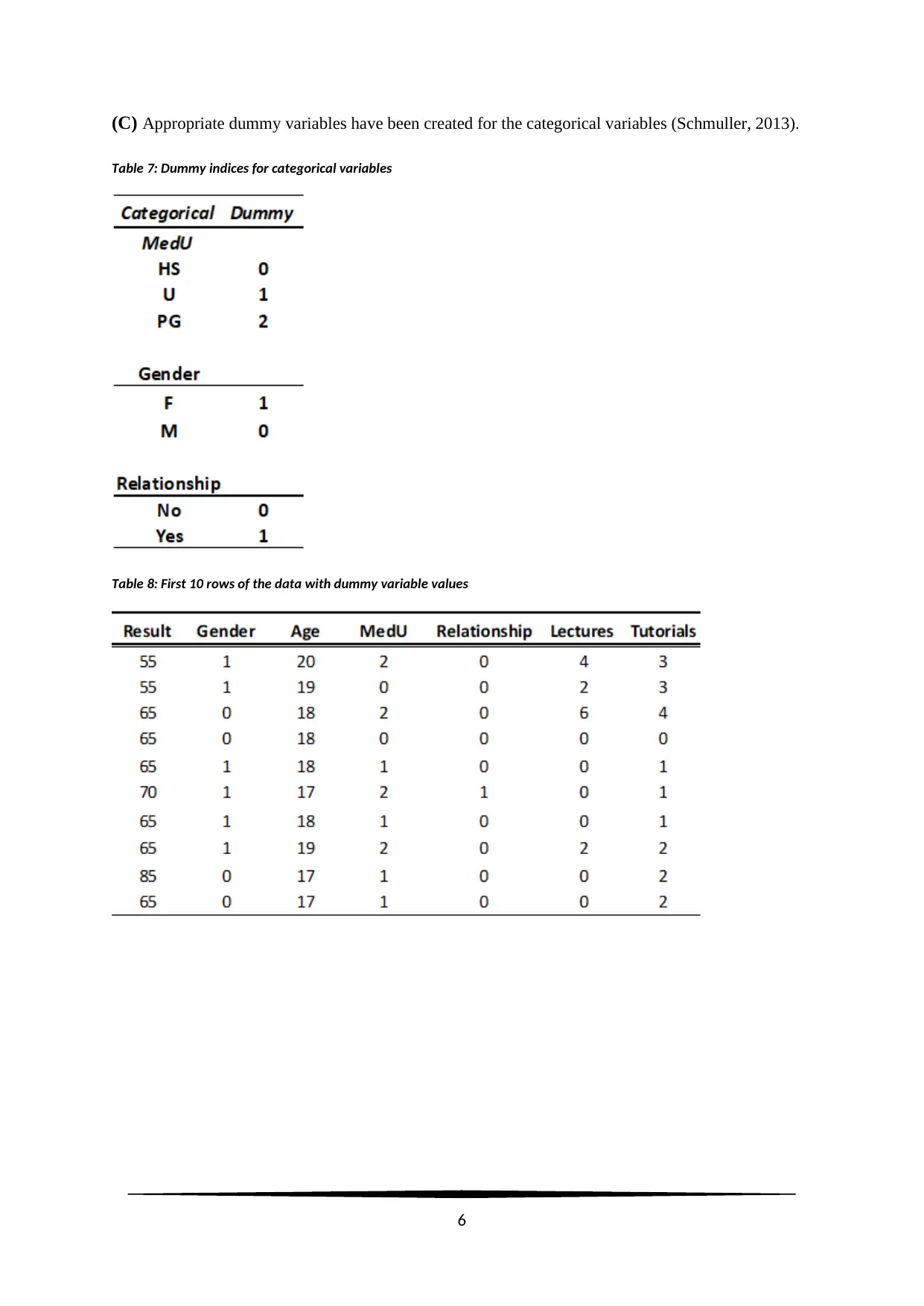
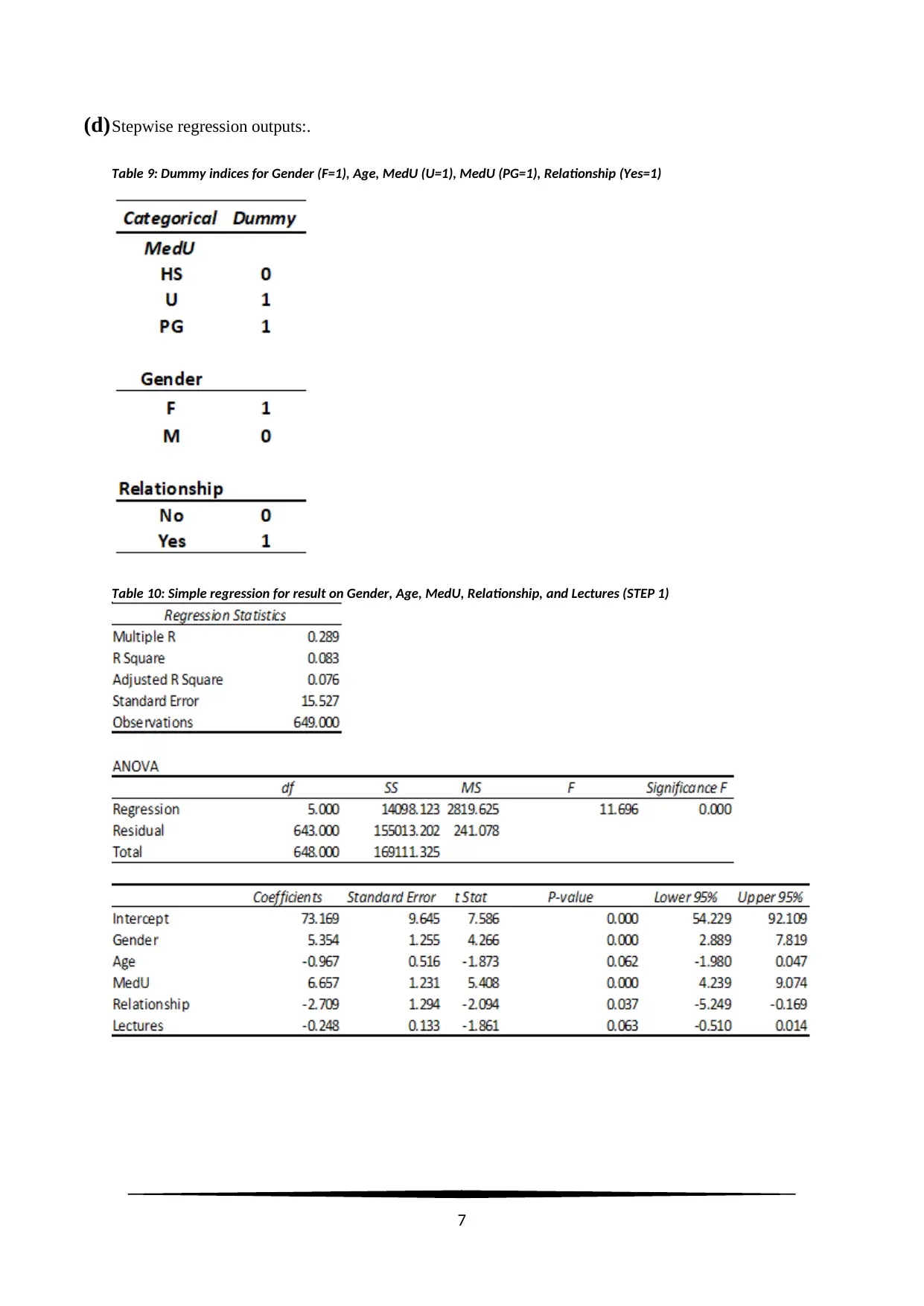
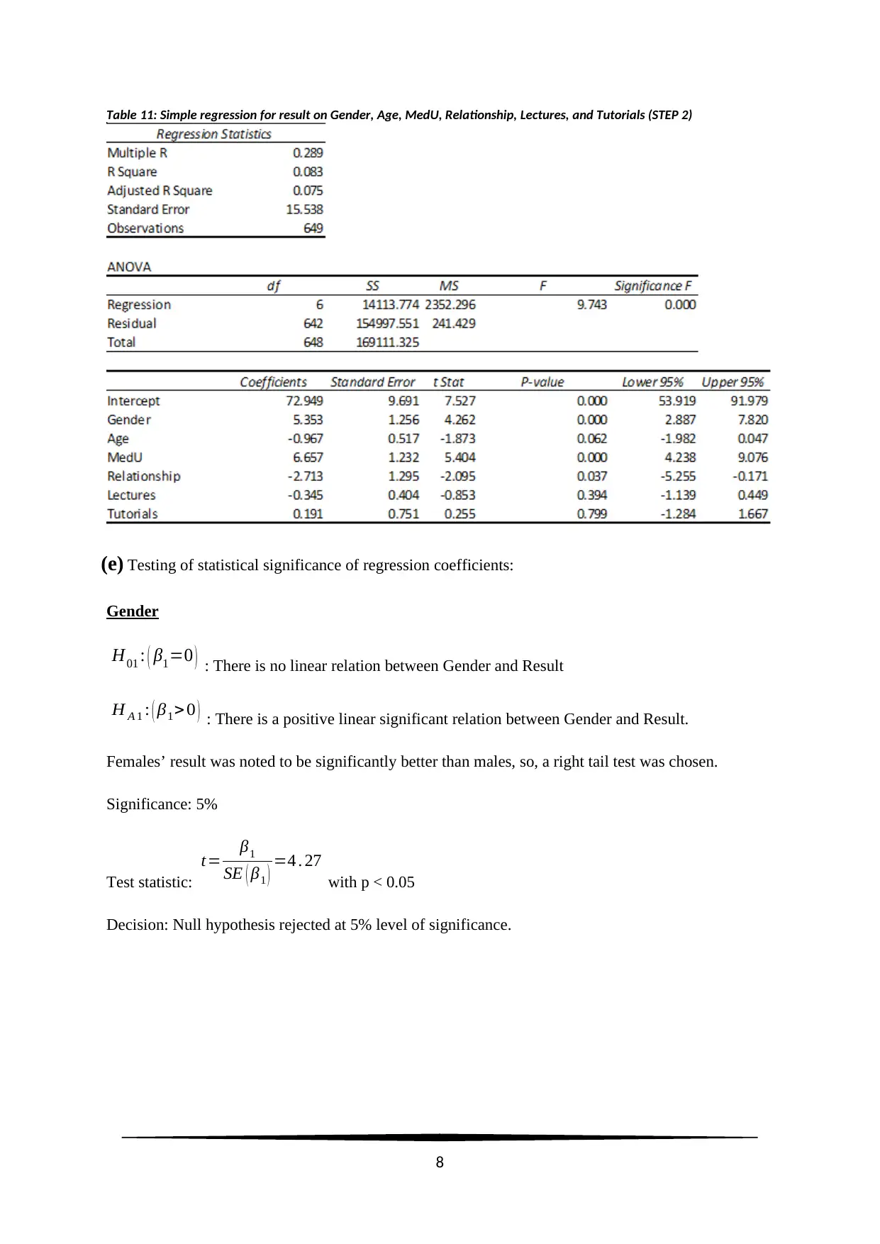
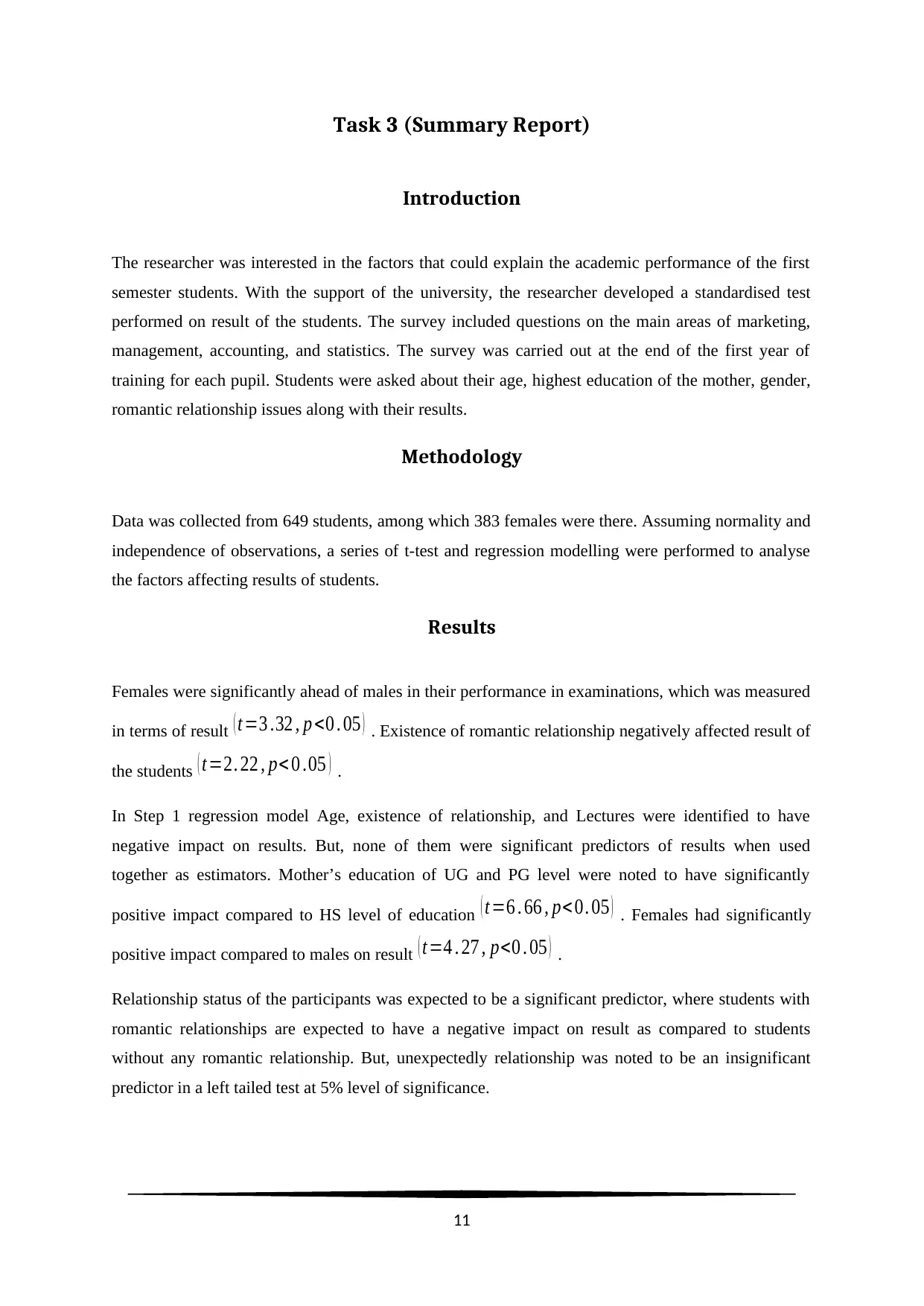
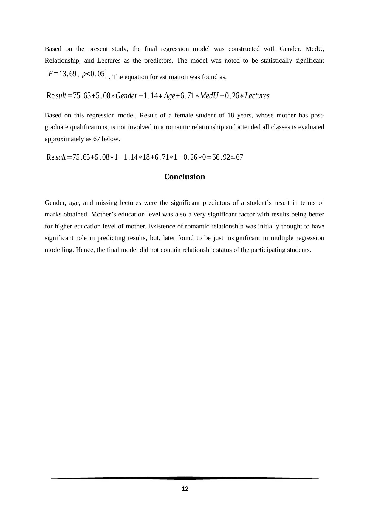
This report analyzes a dataset of 649 first-year business students to identify factors influencing their academic performance in a standardized test. The study employs t-tests and regression modeling to examine the impact of variables like gender, age, mother's education, romantic relationship status, lecture attendance, and tutorial attendance on student results. Key findings include that females performed significantly better than males, and the existence of a romantic relationship had a negative impact on results. The final regression model, statistically significant, included gender, mother's education level, relationship status, and lectures as predictors. The report concludes that gender, age, and lecture attendance were significant predictors, along with mother's education level, while the existence of a romantic relationship was found to be insignificant in the multiple regression model.

BSB123 Data Analysis
1

Task 1
(a) A side-by-side box plot of result is in Figure 1. (Lem, Onghena, Verschaffel, & Van Dooren, 2013).
Figure 1: Distribution of results for males and females
The median of results for females is noted to be at 60, and the distribution of results is noted to be
almost normally distributed with a slight negative skewness implying presence of few girls with
higher results. Third quartile was around 70 signifying that score above which the top 25% females
scored. Hence the mid 50% females scored between 50 and 70.
Median of results for males is 55, and the distribution of results is noted to be almost normally
distributed with a slight negative skewness implying presence of some males with higher results.
Third quartile was around 65 signifying that score above which the top 25% males scored. Hence the
mid 50% males scored between 50 and 65. Therefore, on an average females are observed to fare
better compared to males (Devore, & Berk, 2012).
(b) Normality and independence was assumed. Homogeneity of the dependent variable was checked
using an F-test (Kim, 2015).
H 0: ( μM =μF ) : Average results for males and females are statistically same:
H 0: ( μF ≠μM ) : Average result for females is significantly different than that of the males:
The test is a two tailed test since the difference between the average results is checked.
Significance level: 5%
2

Test statistic:
t= μF−μM
SE ( diff ) =3 . 32
and p < 0.05.
Decision: The null hypothesis is rejected on the basis of p-value.
Table 1: Excel output of the t-test for results between genders
(c) Normality and independence was assumed. Homogeneity of the dependent variable was checked
using an F-test.
H 0: ( μN =μY ) : Average results for both yes and no relationship statuses are statistically same:
H 0: ( μY <μN ) : Average result of students in a romantic relation is significantly lower than that of
the students with no relationship status:
This is the case of a left tailed test.
Significance level: 5%
Test statistic:
t = μN−μY
SE ( diff ) =2 .22
and p < 0.05.
Decision: The null hypothesis is rejected on the basis of p-value.
3

Table 2: Excel output of the t-test for results between two relationship statuses
Task 2
(a) A correlation matrix of Result, Age, Lectures, and Tutorials has been constructed and presented in
Table 5. Very low and negative pairwise correlations between Result and other three variables can
be identified from Table 5. Hence, Age, Lectures, and Tutorials are predictors of Result.
Table 3: Correlation matrix of Result, Age, Lectures, and Tutorials
Correlation Result Age Lectures Tutorials
Result 1
Age -0.107 1
Lectures -0.092 0.152 1
Tutorials -0.084 0.147 0.946 1
(b)
(i)
Table 4: Simple regression for result on age
Regression equation is Results = 86.14 – 1.42 * Age
4

(ii)
Table 5: Simple regression for result on lectures
Regression equation is Results = 60.70 – 0.32* Lectures
(iii)
Table 6: Simple regression for result on tutorials
Regression equation is Results = 61.23 – 0.54* Tutorials
The regression coefficients in the above three linear regression models are noted to be negative and
statistically significant. Therefore, the regression outcomes are in line with the correlation results
(Braun, & Oswald, 2011).
5

(C) Appropriate dummy variables have been created for the categorical variables (Schmuller, 2013).
Table 7: Dummy indices for categorical variables
Table 8: First 10 rows of the data with dummy variable values
6

(d)Stepwise regression outputs:.
Table 9: Dummy indices for Gender (F=1), Age, MedU (U=1), MedU (PG=1), Relationship (Yes=1)
Table 10: Simple regression for result on Gender, Age, MedU, Relationship, and Lectures (STEP 1)
7

Table 11: Simple regression for result on Gender, Age, MedU, Relationship, Lectures, and Tutorials (STEP 2)
(e) Testing of statistical significance of regression coefficients:
Gender
H01 : ( β1=0 ) : There is no linear relation between Gender and Result
H A 1 : ( β1> 0 ) : There is a positive linear significant relation between Gender and Result.
Females’ result was noted to be significantly better than males, so, a right tail test was chosen.
Significance: 5%
Test statistic:
t= β1
SE ( β1 ) =4 . 27
with p < 0.05
Decision: Null hypothesis rejected at 5% level of significance.
8

Age
H02 : ( β2=0 ) : There is no linear relation between Age and Result
H A 2 : ( β2 <0 ) : There is a negative linear significant relation between Gender and Result.
Age has a significantly negative impact on Result, SO, a left tail test was chosen.
Significance: 5%
Test statistic:
t = β2
SE ( β2 ) =−1. 87
with p = 0.12 > 0.05
Decision: Null hypothesis failed to get rejected at 5% level of significance.
MedU
H03 : ( β3=0 ) : There is no linear relation between MedU and Result
H A 3 : ( β3≠0 ) : There is a significant linear relation between Gender and Result.
Impact of MedU on Result was not tested earlier, a two tail test was chosen.
Significance: 5%
Test statistic:
t= β3
SE ( β3 ) =6 . 66
with p < 0.05
Decision: Null hypothesis is rejected at 5% level of significance.
Relationship
H04 : ( β4=0 ) : There is no linear relation between Relationship and Result
H A 4 : ( β4 <0 ) : There is a negative linear significant relation between Relationship and Result.
Relationship was noted to have significantly effect on result, a left tail test was chosen.
Significance: 5%
Test statistic:
t= β4
SE ( β4 ) =−2. 09
with p = 0.074
9

Decision: Null hypothesis failed to get rejected at 5% level of significance.
Lectures
H05 : ( β5=0 ) : There is no linear relation between Lectures and Result
H A 5 : ( β5 <0 ) : There is a negative linear significant relation between Lectures and Result.
Lectures were noted have a significantly negative impact on Result, a left tail test was chosen.
Significance: 5%
Test statistic:
t= β5
SE ( β5 ) =−1. 86
with p = 0.12 > 0.05
Decision: Null hypothesis failed to get rejected at 5% level of significance.
(f) Regression coefficient in simple regression model for estimating Result by Tutorials was negative. As
discussed in correlation section of task 2 (a), a high positive correlation between Tutorials and
Lectures is responsible for the positive regression coefficient for Tutorials (Multicollinearity).
10

Task 3 (Summary Report)
Introduction
The researcher was interested in the factors that could explain the academic performance of the first
semester students. With the support of the university, the researcher developed a standardised test
performed on result of the students. The survey included questions on the main areas of marketing,
management, accounting, and statistics. The survey was carried out at the end of the first year of
training for each pupil. Students were asked about their age, highest education of the mother, gender,
romantic relationship issues along with their results.
Methodology
Data was collected from 649 students, among which 383 females were there. Assuming normality and
independence of observations, a series of t-test and regression modelling were performed to analyse
the factors affecting results of students.
Results
Females were significantly ahead of males in their performance in examinations, which was measured
in terms of result ( t=3 .32 , p <0 . 05 ) . Existence of romantic relationship negatively affected result of
the students ( t=2. 22 , p< 0 .05 ) .
In Step 1 regression model Age, existence of relationship, and Lectures were identified to have
negative impact on results. But, none of them were significant predictors of results when used
together as estimators. Mother’s education of UG and PG level were noted to have significantly
positive impact compared to HS level of education ( t=6 . 66 , p< 0. 05 ) . Females had significantly
positive impact compared to males on result ( t=4 . 27 , p<0 . 05 ) .
Relationship status of the participants was expected to be a significant predictor, where students with
romantic relationships are expected to have a negative impact on result as compared to students
without any romantic relationship. But, unexpectedly relationship was noted to be an insignificant
predictor in a left tailed test at 5% level of significance.
11

Based on the present study, the final regression model was constructed with Gender, MedU,
Relationship, and Lectures as the predictors. The model was noted to be statistically significant
( F=13. 69 , p<0 . 05 ) . The equation for estimation was found as,
Re sult =75 .65+5 . 08∗Gender−1. 14∗Age+6 .71∗MedU −0 .26∗Lectures
Based on this regression model, Result of a female student of 18 years, whose mother has post-
graduate qualifications, is not involved in a romantic relationship and attended all classes is evaluated
approximately as 67 below.
Re sult =75 .65+5 . 08∗1−1 .14∗18+6 . 71∗1−0 .26∗0=66 . 92≃67
Conclusion
Gender, age, and missing lectures were the significant predictors of a student’s result in terms of
marks obtained. Mother’s education level was also a very significant factor with results being better
for higher education level of mother. Existence of romantic relationship was initially thought to have
significant role in predicting results, but, later found to be just insignificant in multiple regression
modelling. Hence, the final model did not contain relationship status of the participating students.
12

References
Braun, M. T., & Oswald, F. L. (2011). Exploratory regression analysis: A tool for selecting models
and determining predictor importance. Behavior research methods, 43(2), 331-339.
Devore, J. L., & Berk, K. N. (2012). Modern mathematical statistics with applications (p. 350). New
York: Springer
Kim, T. (2015). T test as a parametric statistic. Korean Journal Of Anesthesiology, 68(6), 540. doi:
10.4097/kjae.2015.68.6.540
Lem, S., Onghena, P., Verschaffel, L., & Van Dooren, W. (2013). The heuristic interpretation of box
plots. Learning And Instruction, 26, 22-35. doi: 10.1016/j.learninstruc.2013.01.001
Schmuller, J. (2013). Statistical analysis with Excel for dummies (3rd ed.). Hoboken, N.J.: Wiley.
13