Statistics Homework: Exploring Relationships Between BMI and Activity

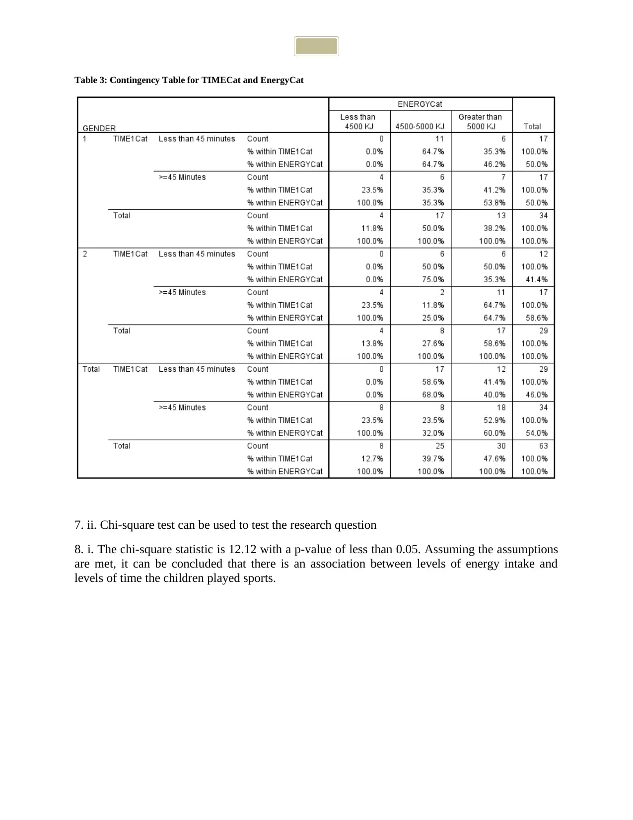
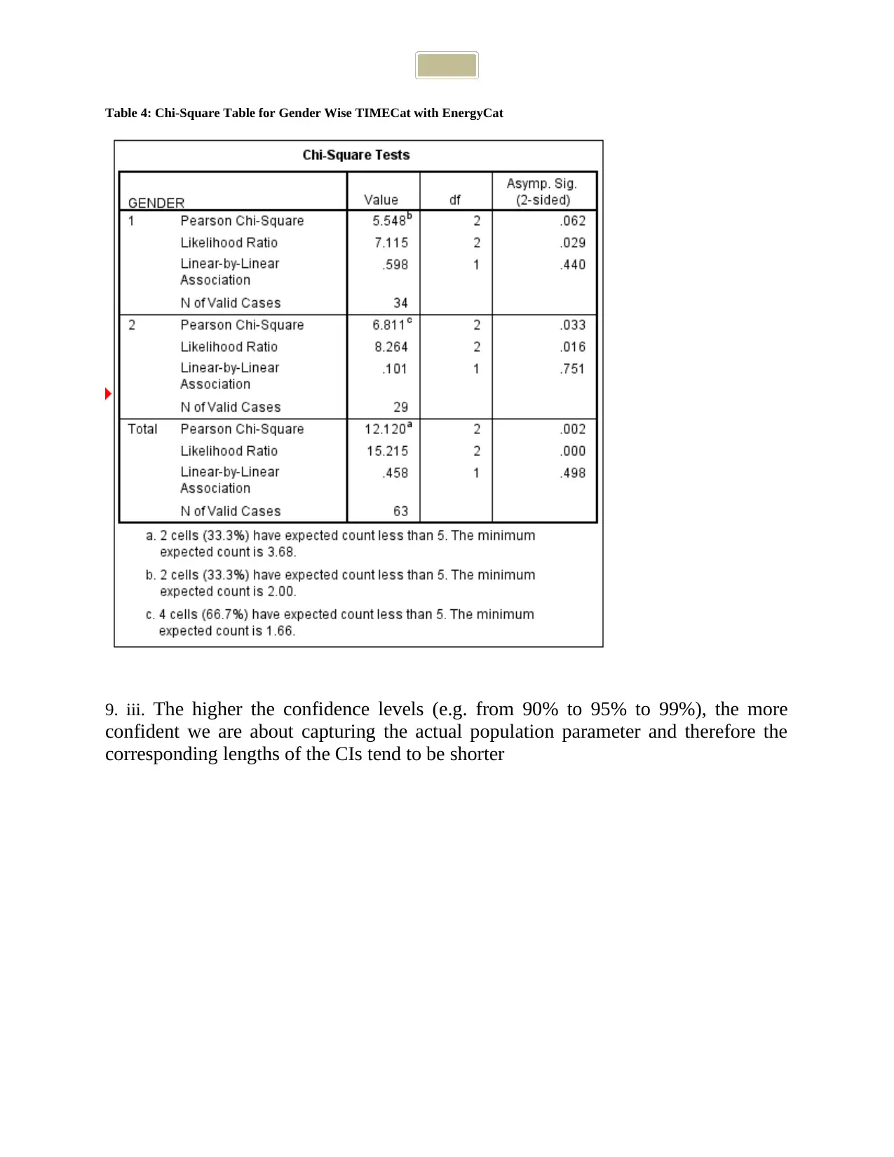
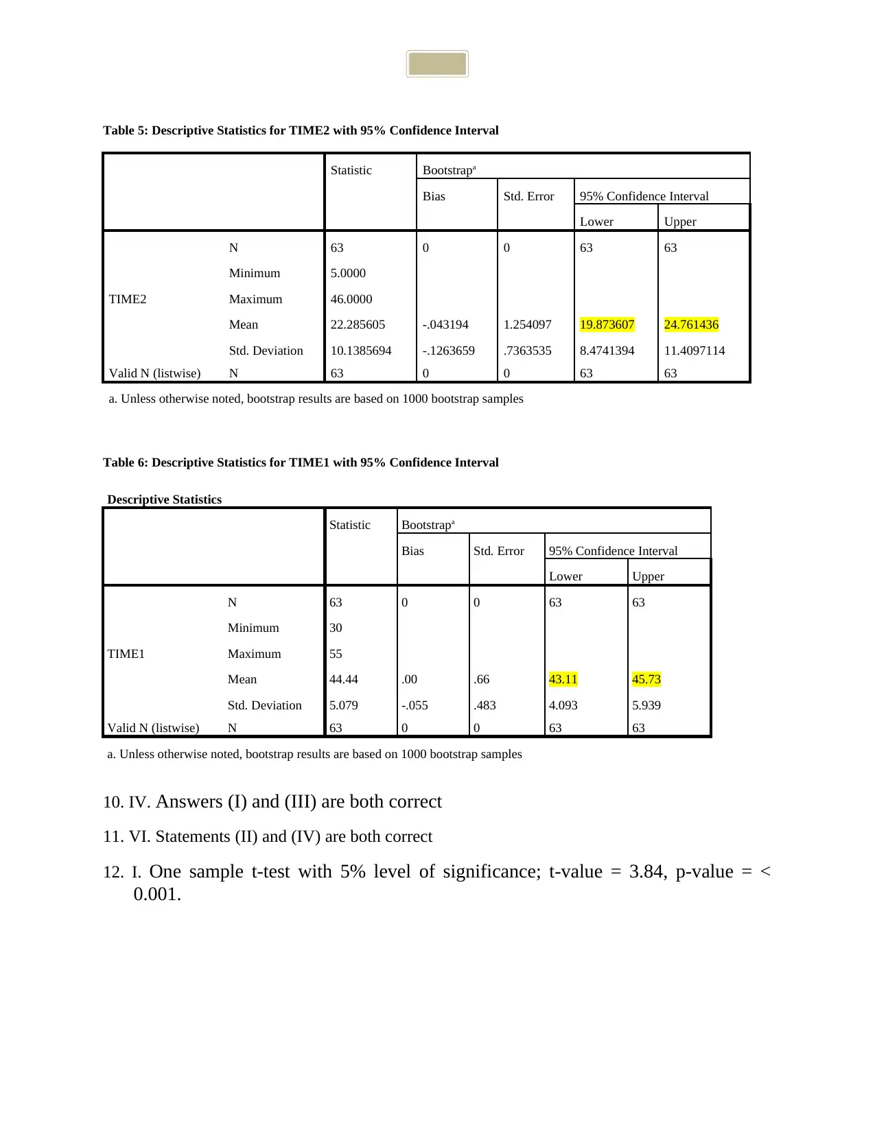
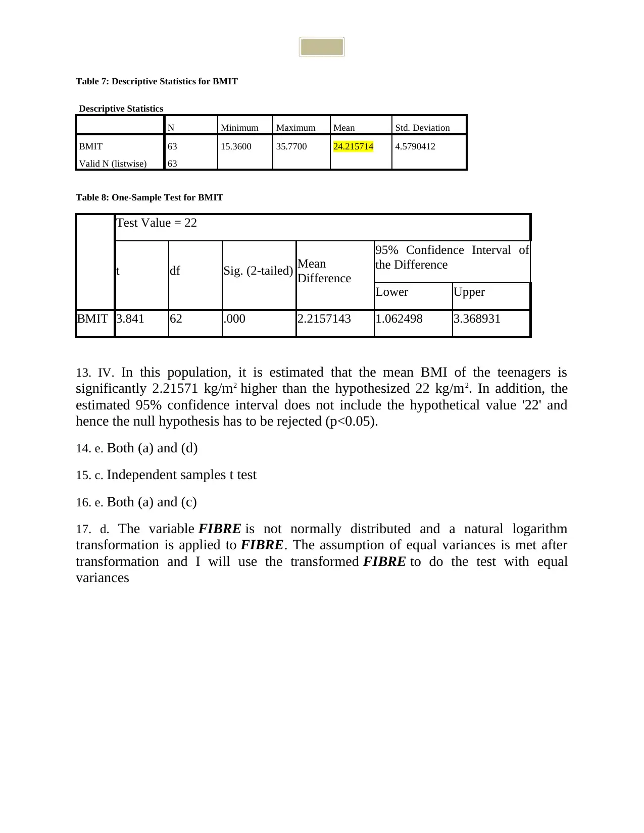
This assignment solution covers a range of statistical analyses related to Body Mass Index (BMI) and sports activity among children and teenagers. It includes descriptive statistics, normality tests, chi-square tests for association, t-tests for comparing means, ANOVA for group comparisons, and regression analysis to predict BMI based on activity levels. The solution provides answers to multiple-choice questions with justifications based on SPSS outputs, addressing topics such as appropriate statistical measures, hypothesis testing, confidence intervals, and the interpretation of statistical results. Outputs generated from SPSS as evidence to support the answers for questions have been provided. The analysis explores relationships between energy intake, time spent playing sports, gender, and BMI, offering a comprehensive overview of statistical methods applied to health-related data. The document is a student contribution available on Desklib, a platform offering AI-based study tools and a wide array of solved assignments and past papers.

Answers of Multiple Choice Questions

Answers
1. c. Median and Interquartile range
2. d. In this sample, the average BMI of the children is 20.27 kg/m2, with a standard deviation of
3.67 kg/m2.
3. iii. No, variable BMIT already has a Normal distribution
Figure 1: Box Plot of BMIT Shows that the Variable is Normal

Table 1: Descriptive Values for BMIT Shows Slight Positive Skewness
Descriptive
Statistic Std.
Error
Mean 24.2157 .57690
95% Confidence Interval for Mean
Lower Bound 23.0625
Upper Bound 25.3689
5% Trimmed Mean 24.1857
Median 23.9100
Variance 20.968
Std. Deviation 4.57904
Minimum 15.36
Maximum 35.77
Range 20.41
Interquartile Range 6.64
Skewness .168 .302
Kurtosis -.481 .595
Table 2: Tests of Normality for BMIT
Kolmogorov-Smirnova Shapiro-Wilk
Statistic df Sig. Statistic df Sig.
BMIT .078 63 .200* .986 63 .686
*. This is a lower bound of the true significance.
a. Lilliefors Significance Correction

Figure 2: Q-Q Plot for BMIT Shows that BMIT is Normal
4. i. Mean and standard deviation. The reason is that variable BMIT has a normal (symmetric)
distribution.
5. IV. 90% of the children in this sample had their BMI ranged from 15.06 (mean-2SD) to 33.37
(mean+2SD) kg/m2
6. IV. Of the children who consumed more than 5000 kJ, more of them also tend to spend more
than 45 minutes playing sports (60%).

Table 3: Contingency Table for TIMECat and EnergyCat
7. ii. Chi-square test can be used to test the research question
8. i. The chi-square statistic is 12.12 with a p-value of less than 0.05. Assuming the assumptions
are met, it can be concluded that there is an association between levels of energy intake and
levels of time the children played sports.

Table 4: Chi-Square Table for Gender Wise TIMECat with EnergyCat
9. iii. The higher the confidence levels (e.g. from 90% to 95% to 99%), the more
confident we are about capturing the actual population parameter and therefore the
corresponding lengths of the CIs tend to be shorter

Table 5: Descriptive Statistics for TIME2 with 95% Confidence Interval
Statistic Bootstrapa
Bias Std. Error 95% Confidence Interval
Lower Upper
TIME2
N 63 0 0 63 63
Minimum 5.0000
Maximum 46.0000
Mean 22.285605 -.043194 1.254097 19.873607 24.761436
Std. Deviation 10.1385694 -.1263659 .7363535 8.4741394 11.4097114
Valid N (listwise) N 63 0 0 63 63
a. Unless otherwise noted, bootstrap results are based on 1000 bootstrap samples
Table 6: Descriptive Statistics for TIME1 with 95% Confidence Interval
Descriptive Statistics
Statistic Bootstrapa
Bias Std. Error 95% Confidence Interval
Lower Upper
TIME1
N 63 0 0 63 63
Minimum 30
Maximum 55
Mean 44.44 .00 .66 43.11 45.73
Std. Deviation 5.079 -.055 .483 4.093 5.939
Valid N (listwise) N 63 0 0 63 63
a. Unless otherwise noted, bootstrap results are based on 1000 bootstrap samples
10. IV. Answers (I) and (III) are both correct
11. VI. Statements (II) and (IV) are both correct
12. I. One sample t-test with 5% level of significance; t-value = 3.84, p-value = <
0.001.

Table 7: Descriptive Statistics for BMIT
Descriptive Statistics
N Minimum Maximum Mean Std. Deviation
BMIT 63 15.3600 35.7700 24.215714 4.5790412
Valid N (listwise) 63
Table 8: One-Sample Test for BMIT
Test Value = 22
t df Sig. (2-tailed) Mean
Difference
95% Confidence Interval of
the Difference
Lower Upper
BMIT 3.841 62 .000 2.2157143 1.062498 3.368931
13. IV. In this population, it is estimated that the mean BMI of the teenagers is
significantly 2.21571 kg/m2 higher than the hypothesized 22 kg/m2. In addition, the
estimated 95% confidence interval does not include the hypothetical value '22' and
hence the null hypothesis has to be rejected (p<0.05).
14. e. Both (a) and (d)
15. c. Independent samples t test
16. e. Both (a) and (c)
17. d. The variable FIBRE is not normally distributed and a natural logarithm
transformation is applied to FIBRE. The assumption of equal variances is met after
transformation and I will use the transformed FIBRE to do the test with equal
variances

Figure 3: Box Plot for FIBRE Shows Skewness and Outliers
Table 9: Test of Normality for FIBRE AND LN_FIBRE
Kolmogorov-Smirnov Shapiro-Wilk
Statistic df Sig. Statistic df Sig.
FIBRE .240 63 .000 .773 63 .000
LN_FIBR
E .090 63 .200* .954 63 .020

Table 10: Test of Homogeneity of Variances for the two Genders
LN_FIBRE
Levene
Statistic
df1 df2 Sig.
2.018 1 61 .161
18. I. The test statistics is 2.10, the p-value is 0.04, the 95% CI of the difference is
(0.02, 0.93) and does not include ‘0’, suggesting that we have to reject the null
hypothesis and conclude that the population mean fiber intake is different between the
boys and the girls.
Table 11: Descriptive Statistics for LN_FIBRE
Group Statistics
GENDER N Mean Std. Deviation Std. Error Mean
LN_FIBRE 1 34 1.818076 .9886904 .1695590
2 29 1.339196 .7855503 .1458730
Table 12: Independent Sample t-test for LN_FIBRE for Two Genders
19. d. H0: μchildren - μteenagers = 0, HA: μchildren - μteenagers ≠ 0
20. b. Paired samples t test
21. II. The mean difference between the time the children played sports and the time
the teenagers played sports is 22.16 minutes. The t-value is 14.07, p-value is <0.001,
95% CI of the difference is (19.0, 25.3) minutes and does not include ‘0’, suggesting

that, in this population, there is a significant difference between the time the children
spent playing sports and the time they played sports when they became teenagers.
Table 13: Paired Samples Statistics
Mean N Std. Deviation Std. Error Mean
Pair 1 TIME1 44.44 63 5.079 .640
TIME2 22.285605 63 10.1385694 1.2773397
Table 14: Paired Samples Correlations
N Correlation Sig.
Pair 1 TIME1 & TIME2 63 -.269 .033
Table 15: Paired Samples t-test for TIME1 and TIME2
22. IV. Pearson correlation with 5% level of significance
23. IV. The correlation coefficient (-0.09) indicates that there is a weak negative
relationship between the children’s energy intake and BMI of the teenagers,
suggesting that there is no relationship between energy intake and the BMI of the
teenagers in this population (p = 0.506).

Table 16: Pearson’s Correlations for ENERGY and BMIT
ENERGY BMIT
ENERGY
Pearson Correlation 1 -.085
Sig. (2-tailed) .506
N 63 63
BMIT
Pearson Correlation -.085 1
Sig. (2-tailed) .506
N 63 63
24. V. One-way ANOVA with 5% level of significance
25. V. The F test-statistic is 1.08, p-value is 0.347, suggesting that there are no
significant population mean BMI differences across the groups of children who had
different levels of energy intake
Table 17: One-Way ANOVA for BMIC
Sum of Squares df Mean Square F Sig.
Between Groups 28.880 2 14.440 1.077 .347
Within Groups 804.811 60 13.414
Total 833.691 62
26. e. Both (a) and (d) are correct.
27. e. Both (b) and (c) are correct
28. d. As the p-value (p=0.283) is greater than the level of significance (i.e. 0.05), the null
hypothesis is accepted and it can be concluded that there is no association between time spent
playing sports and children's area of residence in the study population.