BE01106 Business Statistics Assignment: Comprehensive Analysis

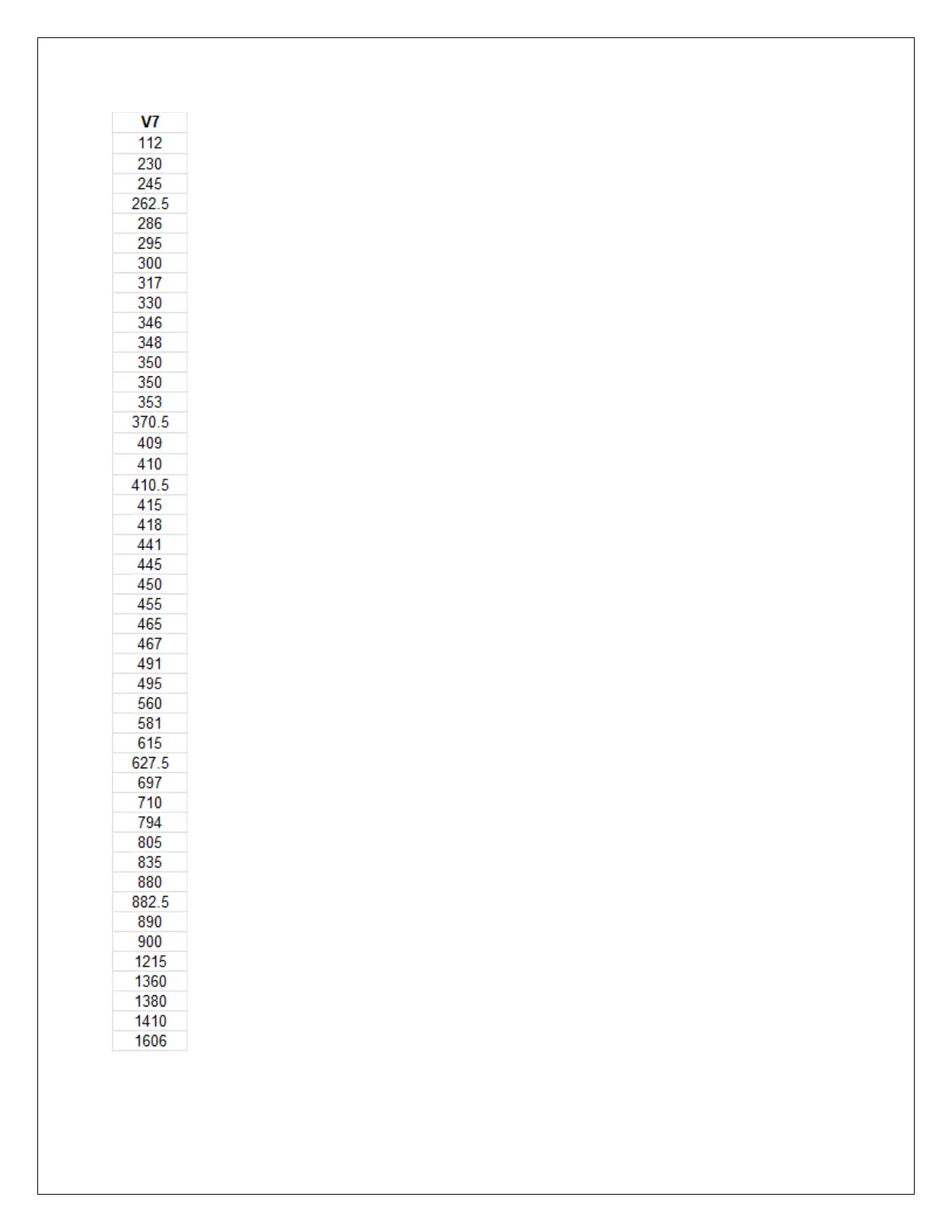
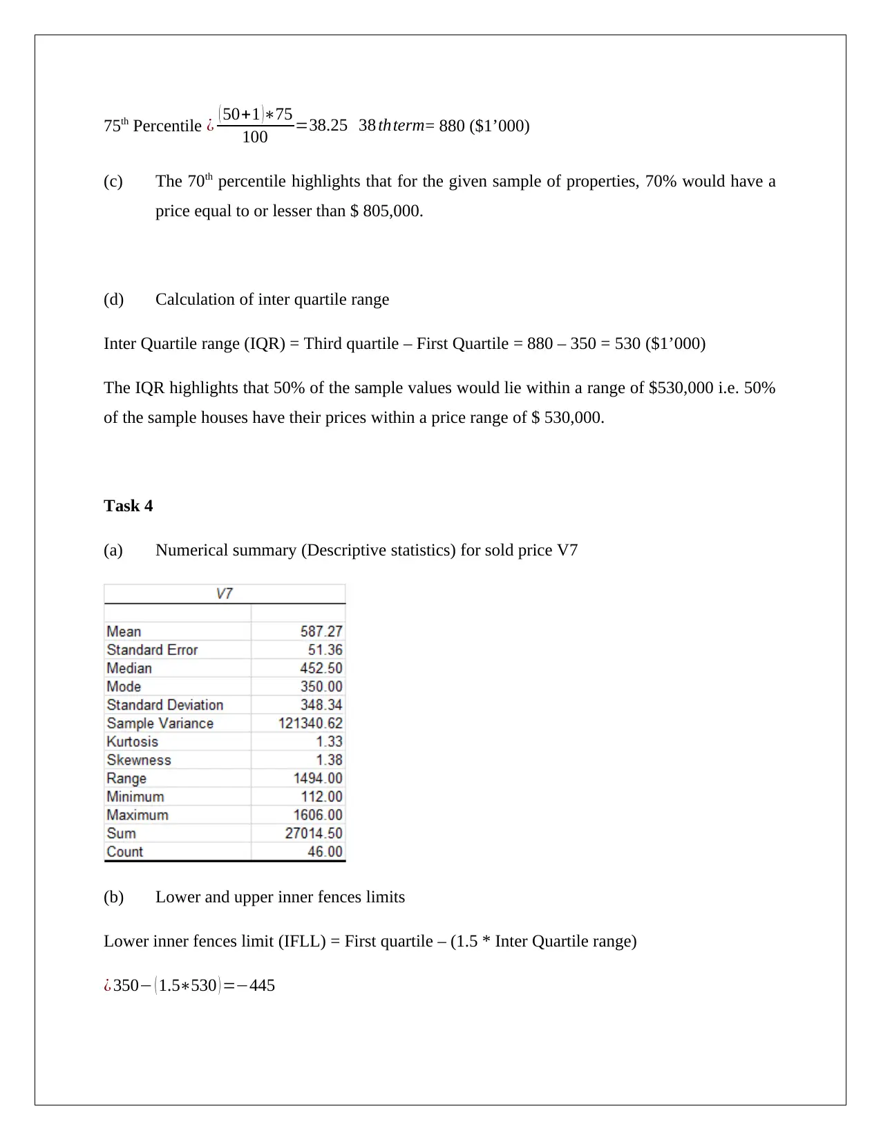
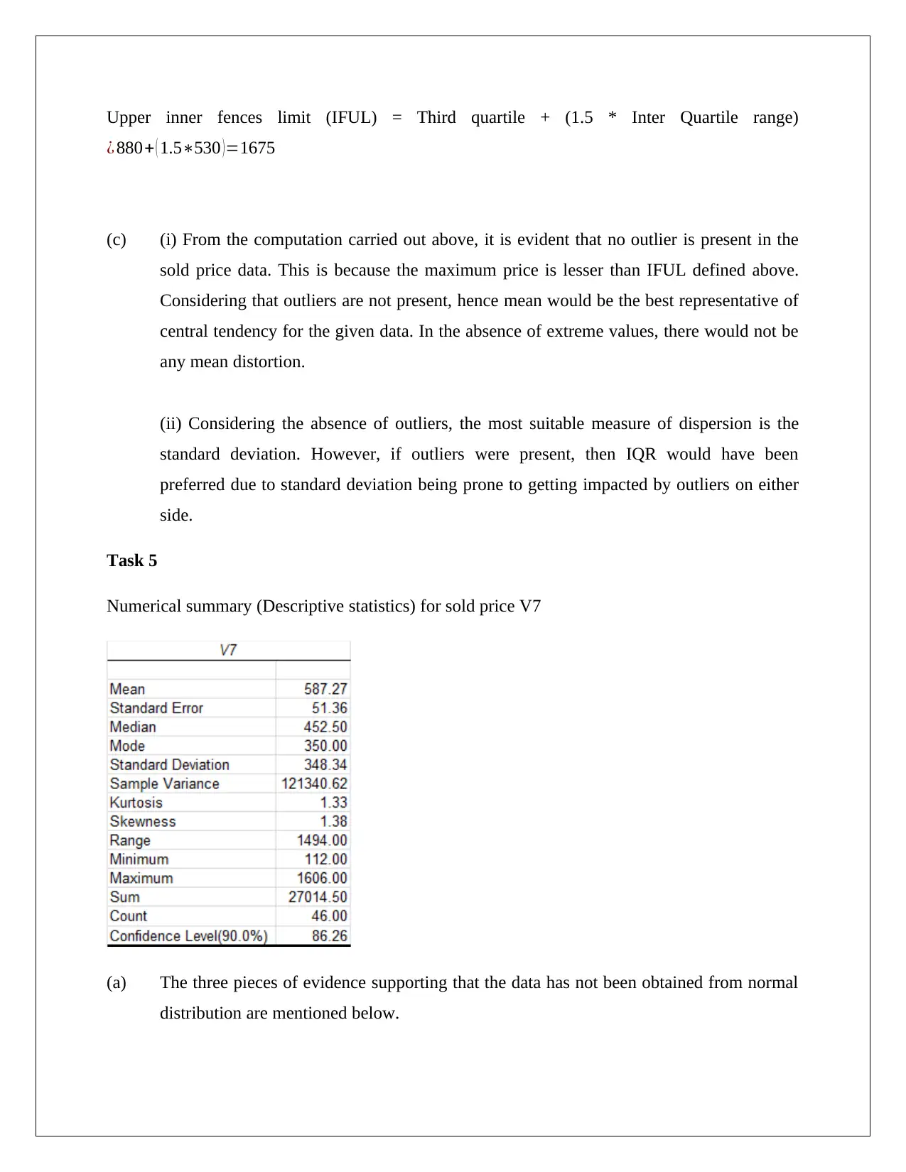
This assignment solution for BE01106 Business Statistics covers a range of statistical analyses. It includes frequency distribution analysis for building types, sorted data analysis for sold prices including percentile calculations such as the 70th percentile, first and third quartiles, and interquartile range. The solution also provides numerical summaries and descriptive statistics for sold prices, identifies the absence of outliers using inner fence limits, and discusses the appropriateness of mean and standard deviation as measures of central tendency and dispersion. Furthermore, it examines the non-normality of the data, calculates expected observations within z-values, and determines upper and lower limits. Finally, the assignment covers point estimation and confidence interval calculations for mean sold prices and brick veneer properties, comparing different confidence levels and their precision. Desklib offers this and many other solved assignments and past papers to aid students in their studies.

BE01106 BUSINESS STATISTICS
ASSIGNMENT
[Pick the date]
Student Name

ASSIGNMENT PART – I
Student Id: 4598219
Row Number: 19
Column Number:2
Sample data set

ASSIGNMENT PART –II
Task 2
Frequency distribution for buliding type (variable V4)
1: Brick
2: Brick Veneer
3: Weatherboard
4: Vacant Land
Frequency column chart
Relative frequency pie chart

(a) Total number of brick building = 21
(b) Highest frequency has observed for veneer property i.e. 32
(c) The proportion of building of weatherboard type is 0.27.
Task 3
(a) The sorted data for variable sold price (V7)

(b) (i) Calculation of percentile
70th Percentile
Percentile location formula
P=70∧n=50
70th Percentile ¿ ( 50+1 )∗70
100 =35.7 36 thterm= 805 ($1’000)
(ii) First quartile and third quartiles
First quartile
Percentile location formula
P=25∧n=50
First quartile ¿ ( 50+1 )∗25
100 =12.7 13 thterm= 350 ($1’000)
Third quartile
Percentile location formula
P=75∧n=50

75th Percentile ¿ ( 50+1 )∗75
100 =38.25 38 thterm= 880 ($1’000)
(c) The 70th percentile highlights that for the given sample of properties, 70% would have a
price equal to or lesser than $ 805,000.
(d) Calculation of inter quartile range
Inter Quartile range (IQR) = Third quartile – First Quartile = 880 – 350 = 530 ($1’000)
The IQR highlights that 50% of the sample values would lie within a range of $530,000 i.e. 50%
of the sample houses have their prices within a price range of $ 530,000.
Task 4
(a) Numerical summary (Descriptive statistics) for sold price V7
(b) Lower and upper inner fences limits
Lower inner fences limit (IFLL) = First quartile – (1.5 * Inter Quartile range)
¿ 350− ( 1.5∗530 ) =−445

Upper inner fences limit (IFUL) = Third quartile + (1.5 * Inter Quartile range)
¿ 880+ ( 1.5∗530 )=1675
(c) (i) From the computation carried out above, it is evident that no outlier is present in the
sold price data. This is because the maximum price is lesser than IFUL defined above.
Considering that outliers are not present, hence mean would be the best representative of
central tendency for the given data. In the absence of extreme values, there would not be
any mean distortion.
(ii) Considering the absence of outliers, the most suitable measure of dispersion is the
standard deviation. However, if outliers were present, then IQR would have been
preferred due to standard deviation being prone to getting impacted by outliers on either
side.
Task 5
Numerical summary (Descriptive statistics) for sold price V7
(a) The three pieces of evidence supporting that the data has not been obtained from normal
distribution are mentioned below.

 The data as highlighted from the descriptive statistics above has skew present which
should not be the case for a normal distribution.
 Besides, as apparent from the descriptive statistics above, there is non-coincidence of the
central tendency measures which also is not a characteristic of normal distribution.
 Further, the number of values within mean +/- one standard deviation would be found
and compared with the empirical expectation of 68% which is not found to be true for the
given data.
(b) The z value for 1.5 = 0.4322
-1.5 to +1.5 = 0.4322 + 0.4322
-1.5 to +1.5 = 0.8664
Hence, 86.64% of the total observations would be expected to lie between z value of -1.5 and
1.5. Thus, total sold price observations expected = (0.8664)*46 = 40 observations apporximately.
(c) Calculation of upper and lower limit
Upper limit = Mean + (1.5 * Standard deviation) = 587.27 + (1.5*348.34) = 1109.78
Lower limit = Mean – (1.5 * Standard deviation) = 587.27 - (1.5*348.34) = 64.76
Using the above values as the upper and lower limits, it can be seen that there are 40 sold price
observations that tend to lie between the above limits. Hence, the values do match.
Task 6
Numerical summary (Descriptive statistics) for sold price V7

(a) (i) Point estmation for mean = $587.27 ($1’000)
(ii) 90% confidence interval ($1’000)
Lower limit of 90% confidence interval = Mean value – Confidence level
¿ 587.27−86.26=501.02
Upper limit 90% confidence interval = Mean value + Confidence level ¿ 587.27+86.26=673.53
90% confidence interval ($1’000) would be [501.02 673.53].
(iii) From the above, it may be concluded that 95% of the selling prices of properties would lie
between $ 501,020 and $673,530.
(b) Yes, the above confidence interval would be considered satisfactory if the population
mean is $ 650,000 as this value tends to belong to the confidence interval for the
population mean highlighted above.
Task 7
Numerical summary (descriptive statistics) for “brick veneer properties” is highlighted below:

(a) (i) The point estimates for mean = 0.32
(ii) 99% confidence interval ($1’000)
Lower limit of 99% confidence interval = Mean value – Confidence level ¿ 0.32−0.18=0.14
Upper limit 99% confidence interval = Mean value + Confidence level ¿ 0.32+0.18=0.50
99% confidence interval ($1’000) would be [0.14 0.50].
(b) 95% confidence interval ($1’000)
95% confidence interval = (Sample Statistic) + {(Critical z or t) * (Standard Error of the Sample
Statistic)}
Population distribution has given as normal distribution and hence, z value would be taken into
consideration.
The z value for 95% confidence interval = 1.96
Lower limit of 95% confidence interval ¿ ( 0.32 ) − ( 1.96∗0.07 ) =0.19
Upper limit 95% confidence interval ¿ ( 0.32 ) + ( 1.96∗0.07 ) =0.38
95% confidence interval would be [0.19 0.38].