BEO1106 Business Statistics Assignment: In-depth Statistical Analysis

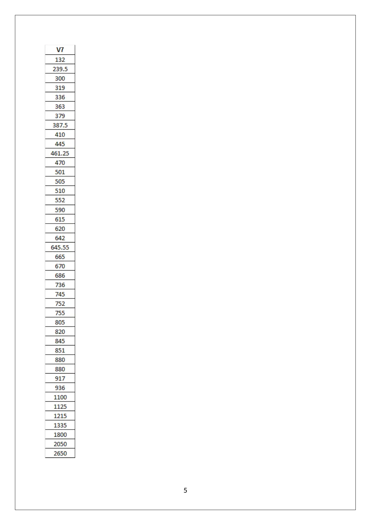
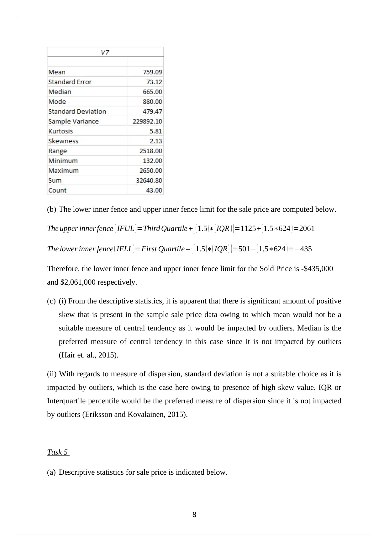
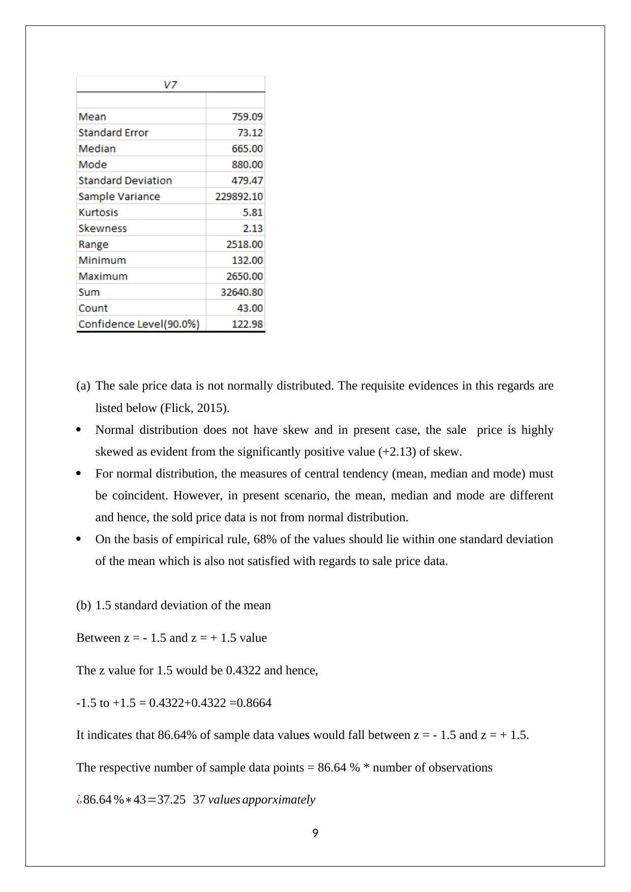
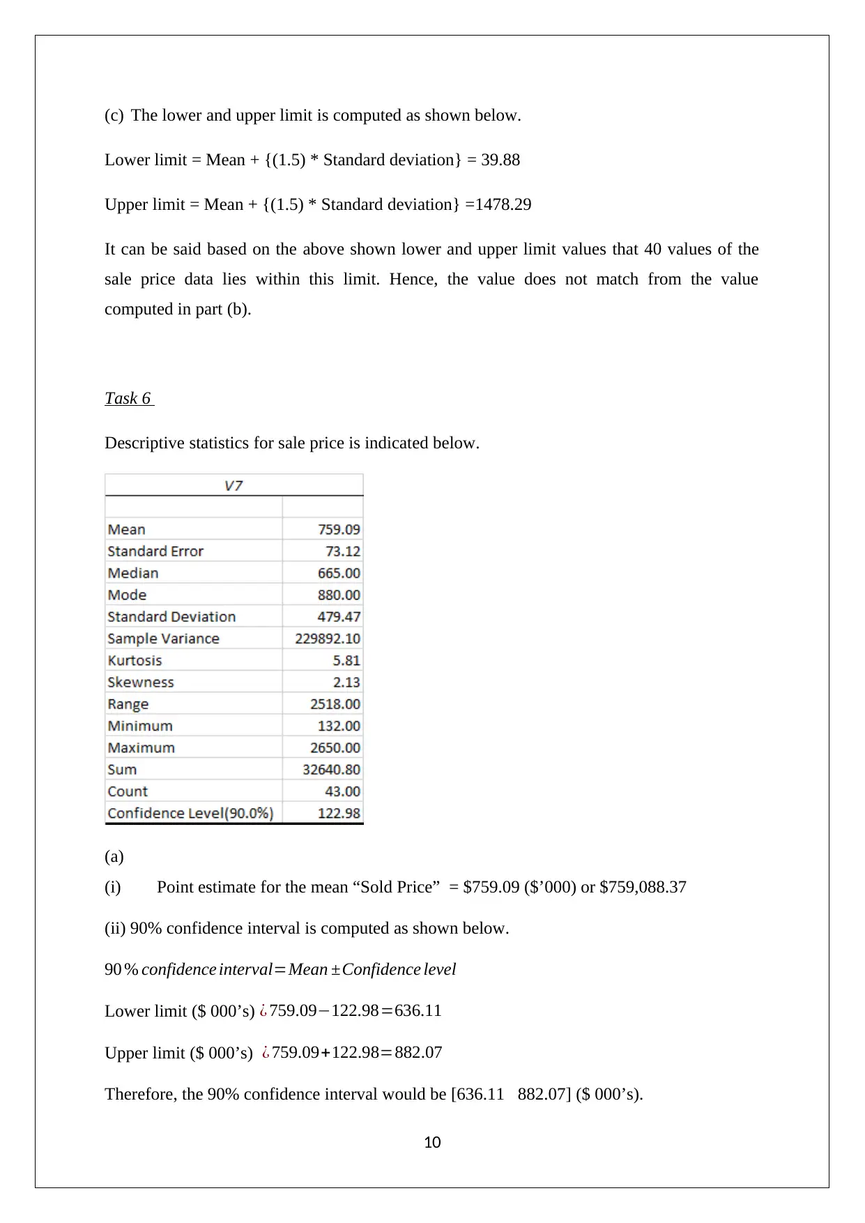
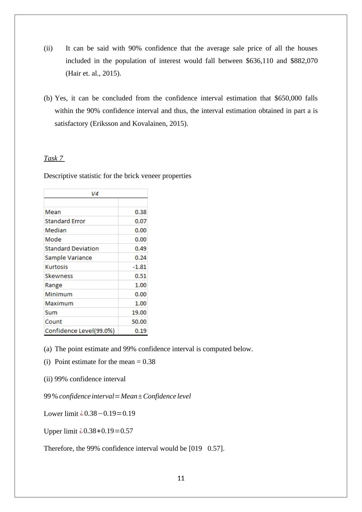
This document presents a comprehensive solution to a business statistics assignment, encompassing various statistical analyses and interpretations. The assignment involves analyzing a sample dataset to determine frequency distributions, calculate percentiles and quartiles, and compute descriptive statistics. It assesses the skewness of the data, identifies appropriate measures of central tendency and dispersion, and evaluates whether the data follows a normal distribution. Furthermore, the solution includes the calculation and interpretation of confidence intervals for the mean sold price and proportions, along with a discussion on the implications of these statistical measures. The assignment leverages statistical formulas and methodologies to derive meaningful insights from the provided data, offering a detailed understanding of statistical concepts and their application in real-world scenarios. Desklib provides access to this and many other solved assignments contributed by students.

BUSINESS STATISTICS
[DATE]

Assignment Part 1
Student Id = 4610559
Last three digits = 559
Column = 5
Row = 59
1

2

Assignment Part II
Task 2
Frequency distribution column chart for building type (V4 variable)
Row Labels Count of V4
1 (Brick) 17
2 (Brick veneer) 19
3 (Weatherboard) 10
4 (Vacant land) 4
Grand Total 50
1 (Brick) 2 (Brick veneer) 3 (Weatherboard) 4 (Vacant land)
0
2
4
6
8
10
12
14
16
18
20
17
19
10
4
Building Type
Building Type
Frequency
Relative frequency pie chart for building type (V4 variable)
3

1 (Brick); 17; 34%
2 (Brick veneer); 19;
38%
3 (Weatherboard);
10; 20%
4 (Vacant land); 4;
8%
Building Type
1 (Brick)
2 (Brick veneer)
3 (Weatherboard)
4 (Vacant land)
(a) Number of brick building in sample = 17
(b) Most frequently occurred building type in sample = Brick veneer
(c) Proportion of total properties that consists weatherboard building in sample =0.20
Task 3
(a) Sorted ‘Sold Price’ data is indicated below.
4

5

(b) Percentile location formula along with the associated rules would be taken into
consideration to determine the following.
(i) 70th percentile
Percentile location formula
Here,
P=70
N=50 ¿
Now,
70 th percentile= ( 50+1 ) × 70
100
¿ 35.7 term 36 term=936($ ' 000)
(ii) The first and third quartile
The first quartile would be 25th percentile.
Percentile location formula
Here,
P=25
N=50 ¿
Now,
25 th percentile= ( 50+1 ) × 25
100
¿ 12.75 term 13th term=501($ ' 000)
6

The third quartile would be 75th percentile.
Percentile location formula
Here,
P=75
N=50 ¿
Now,
75 th percentile= ( 50+1 ) × 75
100
¿ 38.25 term 38 term=1125 ($ ' 000)
(c) The 70th percentile indicates that 70% of the sample property would have sold price same
as or lower than $936,000 (Hillier, 2016).
(d) Inter quartile range or IQR of the sample for sold price data
Inter Quartile Range = Third quartile – First Quartile
Inter Quartile Range=1125−501=624( $' 000)
Inter quartile range is indicative of the aspect that middle 50% of sample properties sold have
prices which would fall within $530,000 range (Flick, 2015).
Task 4
(a) Descriptive statistics for sale price is shown below.
7

(b) The lower inner fence and upper inner fence limit for the sale price are computed below.
The upper inner fence ( IFUL )=Third Quartile + { ( 1.5 )∗ ( IQR ) }=1125+ ( 1.5∗624 )=2061
The lower inner fence ( IFLL ) =First Quartile – { ( 1.5 )∗( IQR ) }=501− ( 1.5∗624 ) =−435
Therefore, the lower inner fence and upper inner fence limit for the Sold Price is -$435,000
and $2,061,000 respectively.
(c) (i) From the descriptive statistics, it is apparent that there is significant amount of positive
skew that is present in the sample sale price data owing to which mean would not be a
suitable measure of central tendency as it would be impacted by outliers. Median is the
preferred measure of central tendency in this case since it is not impacted by outliers
(Hair et. al., 2015).
(ii) With regards to measure of dispersion, standard deviation is not a suitable choice as it is
impacted by outliers, which is the case here owing to presence of high skew value. IQR or
Interquartile percentile would be the preferred measure of dispersion since it is not impacted
by outliers (Eriksson and Kovalainen, 2015).
Task 5
(a) Descriptive statistics for sale price is indicated below.
8

(a) The sale price data is not normally distributed. The requisite evidences in this regards are
listed below (Flick, 2015).
 Normal distribution does not have skew and in present case, the sale price is highly
skewed as evident from the significantly positive value (+2.13) of skew.
 For normal distribution, the measures of central tendency (mean, median and mode) must
be coincident. However, in present scenario, the mean, median and mode are different
and hence, the sold price data is not from normal distribution.
 On the basis of empirical rule, 68% of the values should lie within one standard deviation
of the mean which is also not satisfied with regards to sale price data.
(b) 1.5 standard deviation of the mean
Between z = - 1.5 and z = + 1.5 value
The z value for 1.5 would be 0.4322 and hence,
-1.5 to +1.5 = 0.4322+0.4322 =0.8664
It indicates that 86.64% of sample data values would fall between z = - 1.5 and z = + 1.5.
The respective number of sample data points = 86.64 % * number of observations
¿ 86.64 %∗43=37.25 37 values apporximately
9

(c) The lower and upper limit is computed as shown below.
Lower limit = Mean + {(1.5) * Standard deviation} = 39.88
Upper limit = Mean + {(1.5) * Standard deviation} =1478.29
It can be said based on the above shown lower and upper limit values that 40 values of the
sale price data lies within this limit. Hence, the value does not match from the value
computed in part (b).
Task 6
Descriptive statistics for sale price is indicated below.
(a)
(i) Point estimate for the mean “Sold Price” = $759.09 ($’000) or $759,088.37
(ii) 90% confidence interval is computed as shown below.
90 % confidence interval=Mean ±Confidence level
Lower limit ($ 000’s) ¿ 759.09−122.98=636.11
Upper limit ($ 000’s) ¿ 759.09+122.98=882.07
Therefore, the 90% confidence interval would be [636.11 882.07] ($ 000’s).
10

(ii) It can be said with 90% confidence that the average sale price of all the houses
included in the population of interest would fall between $636,110 and $882,070
(Hair et. al., 2015).
(b) Yes, it can be concluded from the confidence interval estimation that $650,000 falls
within the 90% confidence interval and thus, the interval estimation obtained in part a is
satisfactory (Eriksson and Kovalainen, 2015).
Task 7
Descriptive statistic for the brick veneer properties
(a) The point estimate and 99% confidence interval is computed below.
(i) Point estimate for the mean = 0.38
(ii) 99% confidence interval
99 % confidence interval=Mean ± Confidence level
Lower limit ¿ 0.38−0.19=0.19
Upper limit ¿ 0.38+0.19=0.57
Therefore, the 99% confidence interval would be [019 0.57].
11