PUBH620 Assessment Task 1: Analysis of ACU Student Data

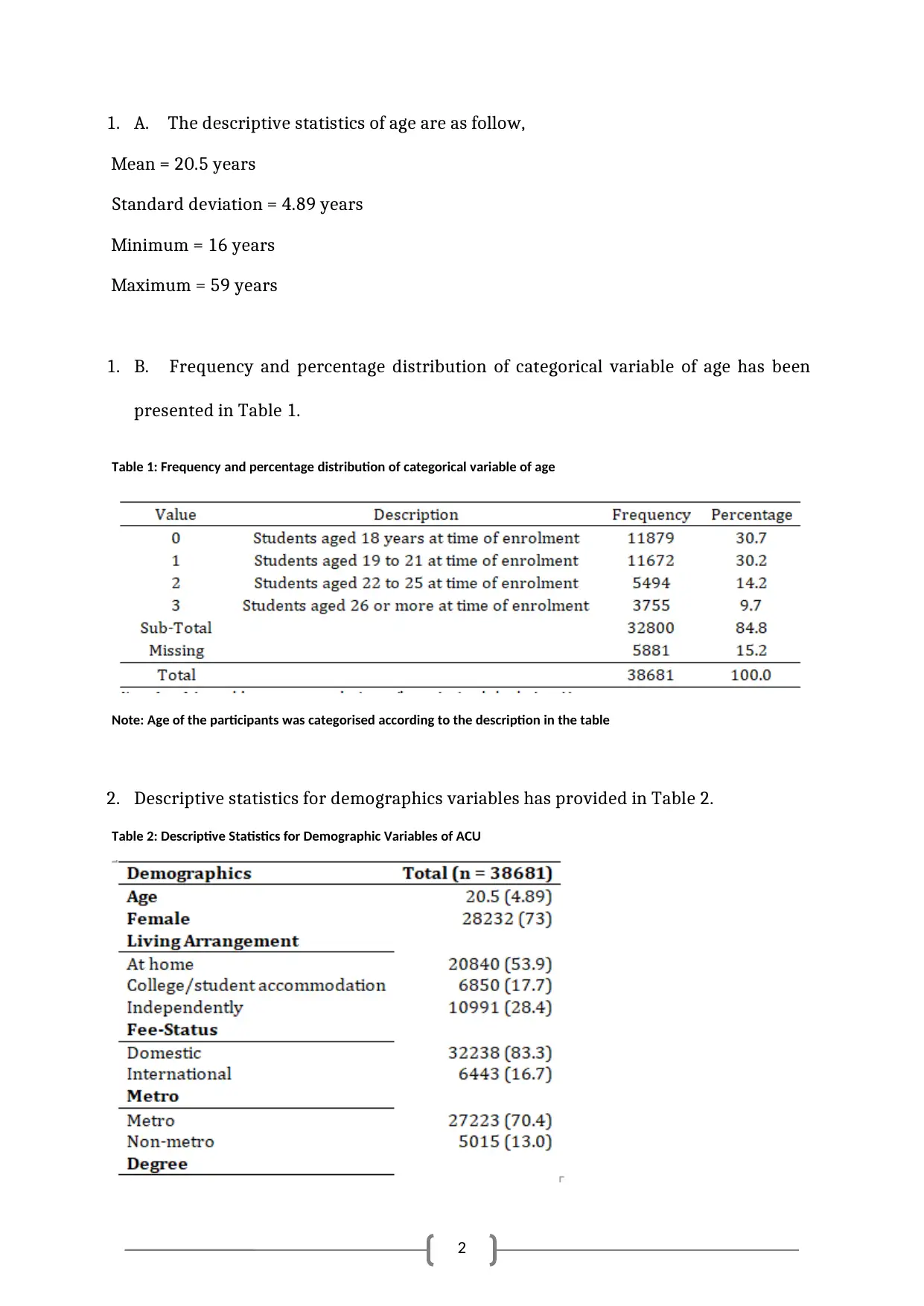
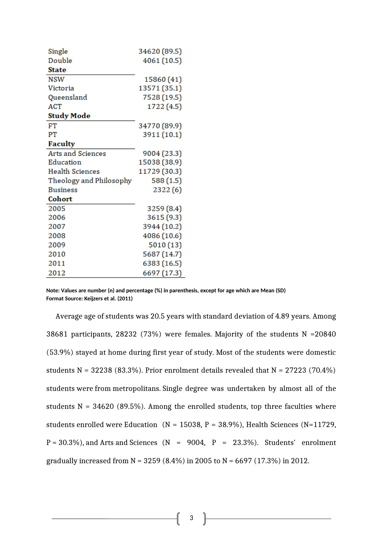
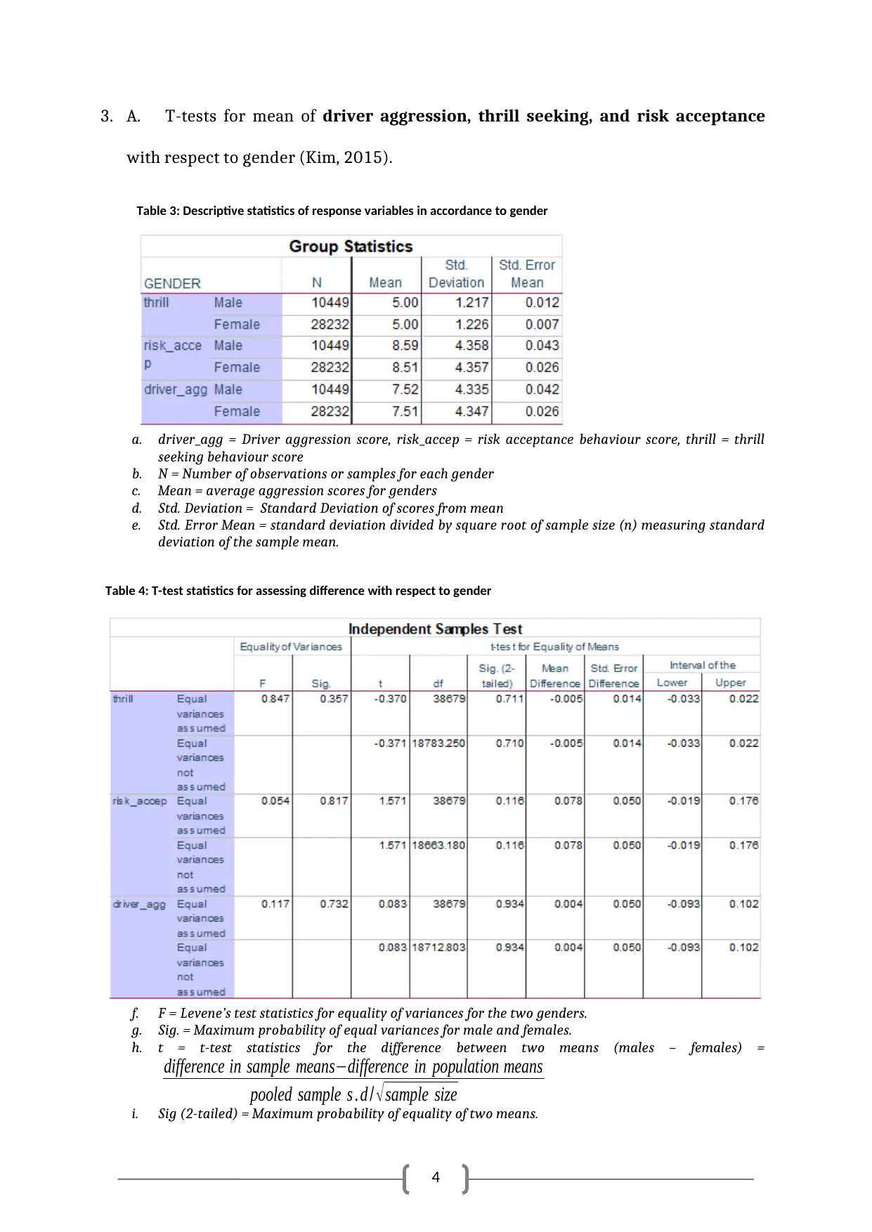
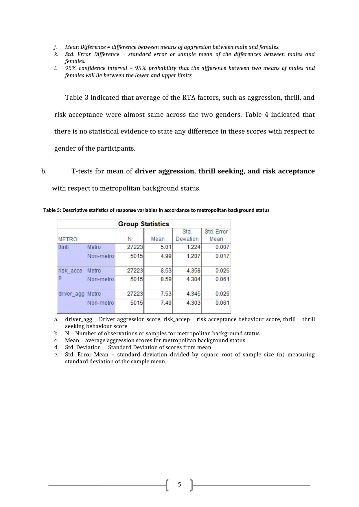
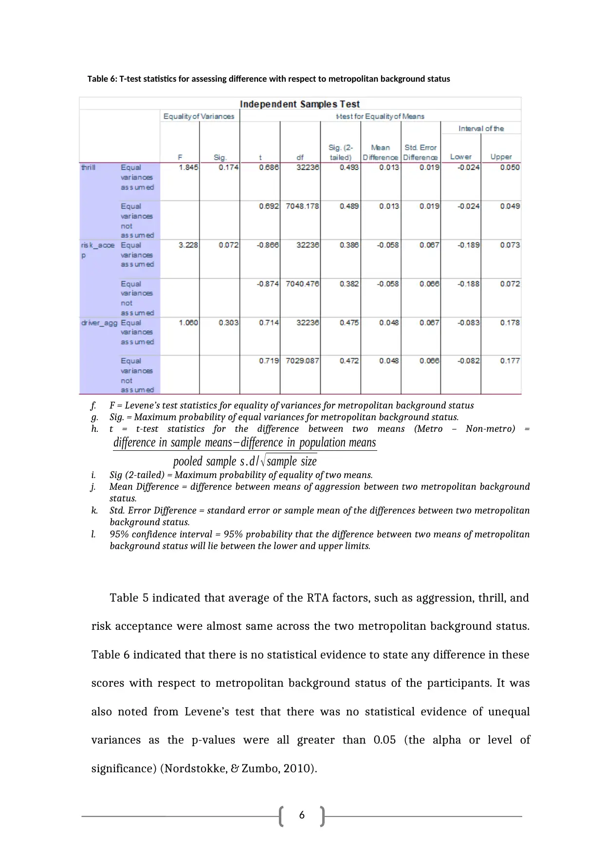
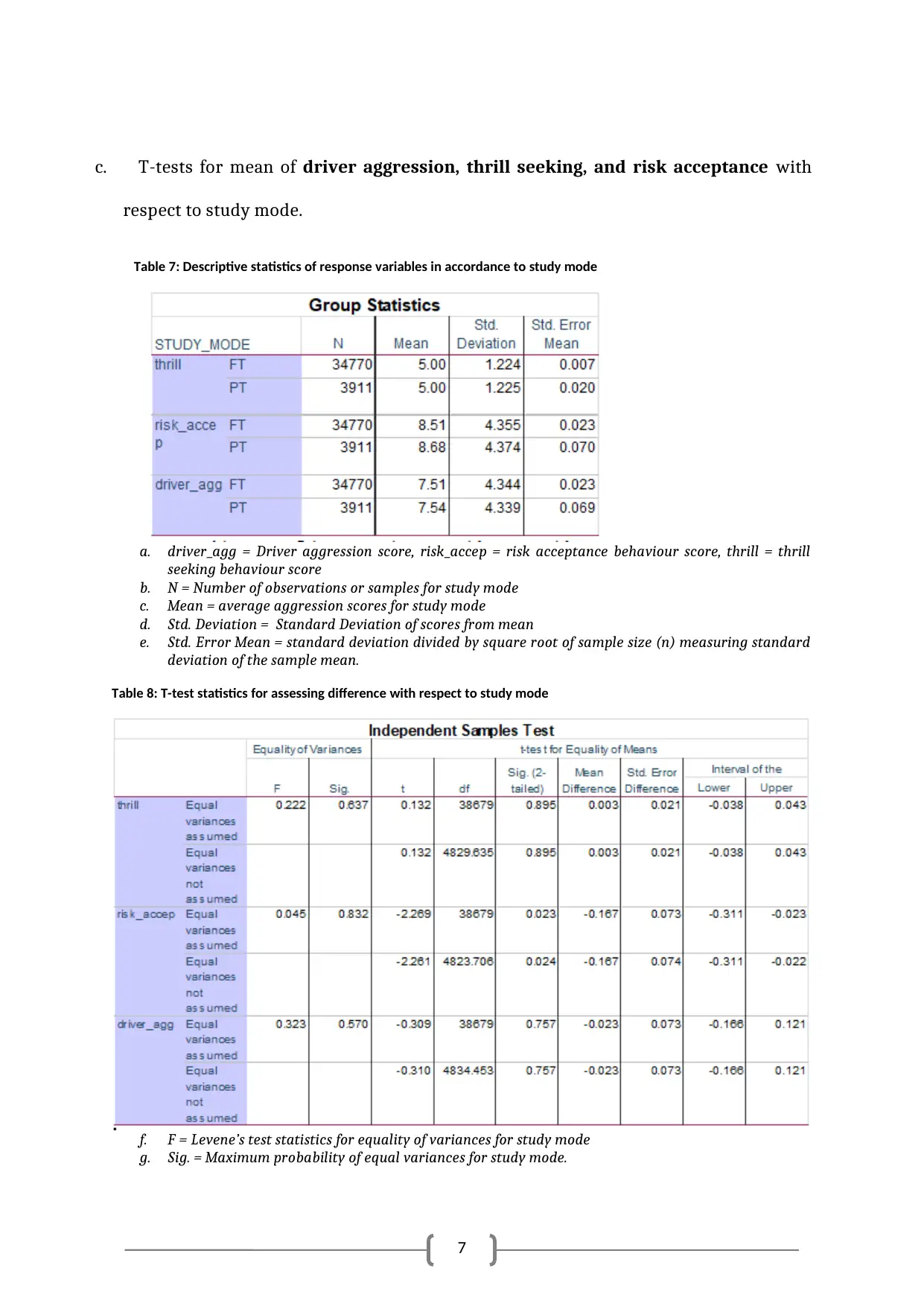
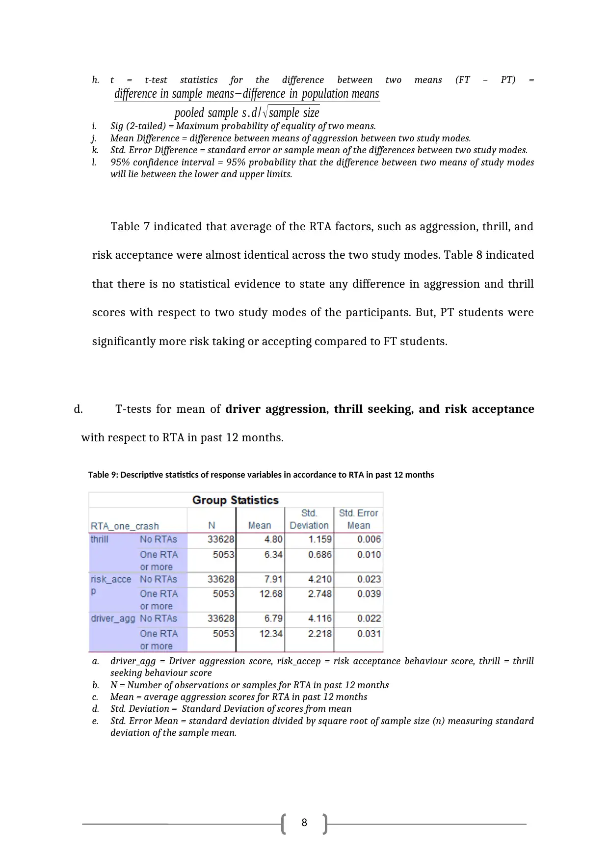
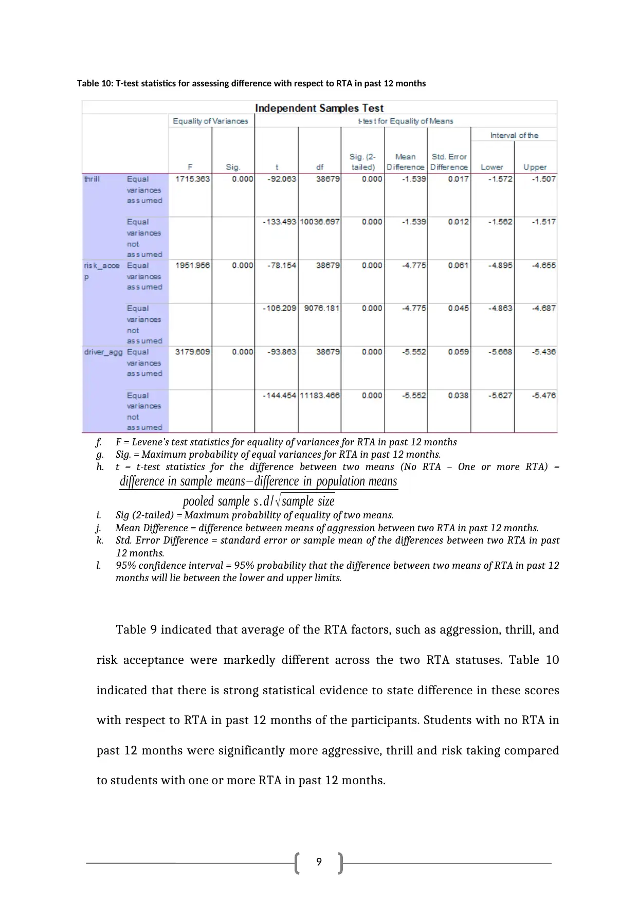
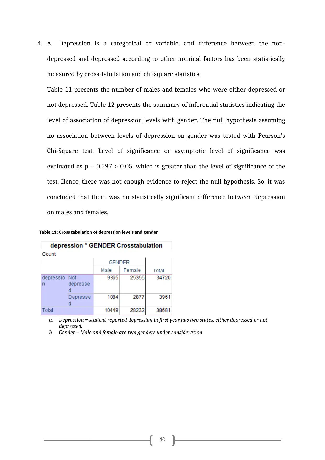
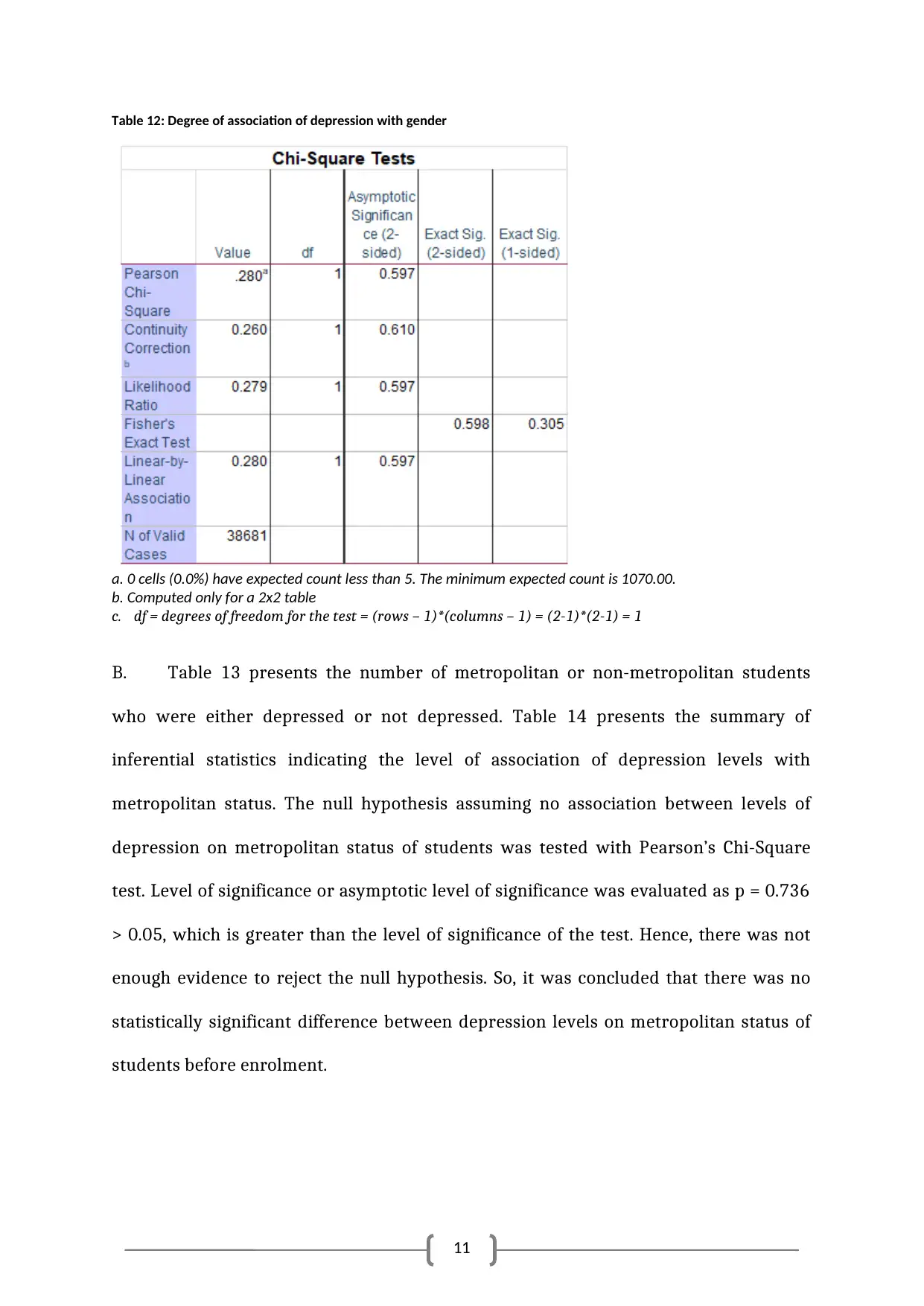
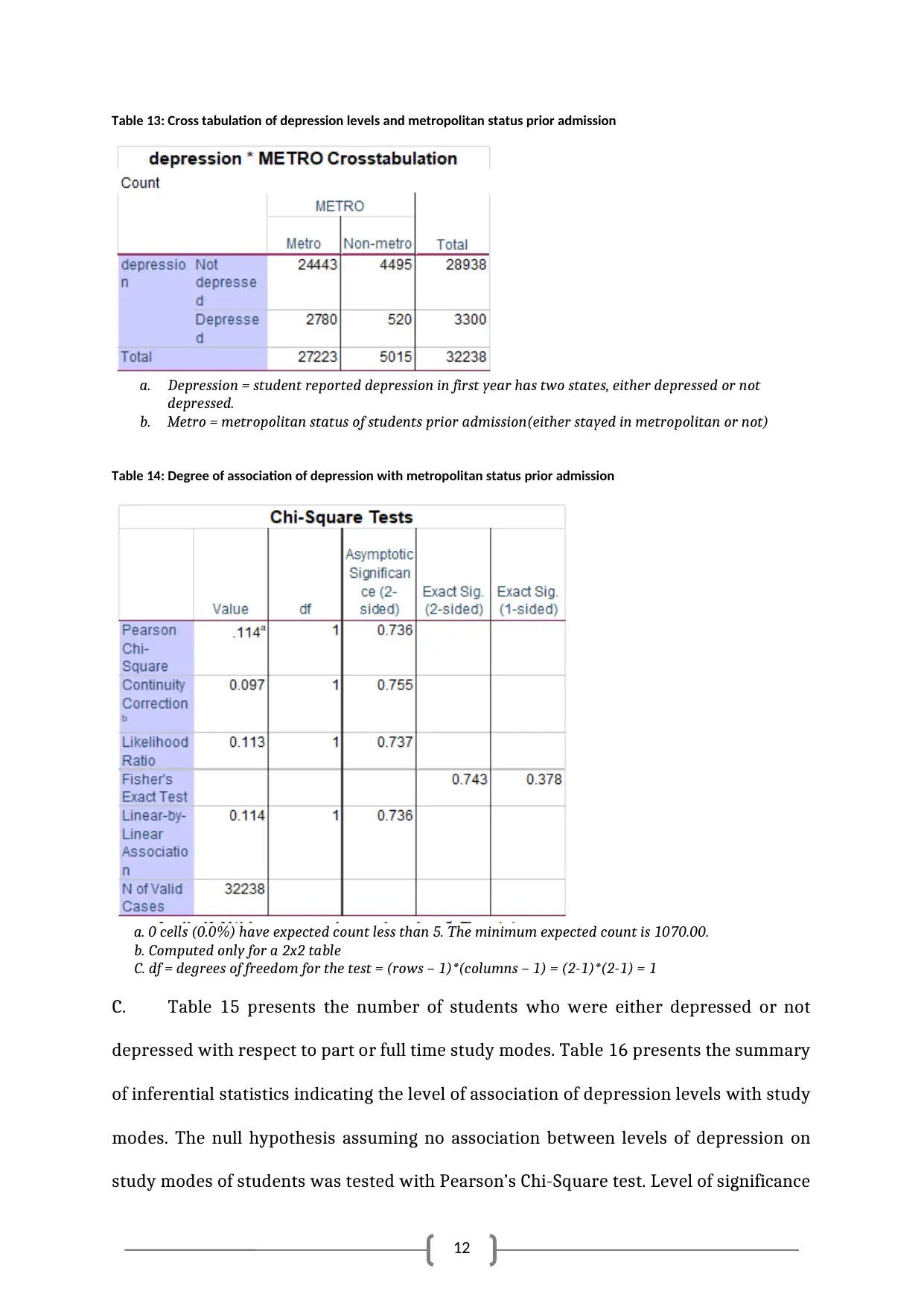
This document presents an analysis of a dataset related to ACU student health and wellbeing, focusing on road traffic accidents, depression, and obesity. The analysis includes descriptive statistics, t-tests, and chi-square tests to examine relationships between various factors such as gender, metropolitan status, study mode, and road traffic accident history. The assignment explores the descriptive statistics of age, demographic variables, and the results of t-tests comparing the means of driver aggression, thrill-seeking, and risk acceptance across different groups. It also investigates the association between depression levels and factors like gender and metropolitan status using cross-tabulation and chi-square tests. The findings indicate no statistically significant differences in depression levels based on gender or metropolitan status, but significant differences in risk-taking behavior based on study mode and prior road traffic accidents. The document provides detailed tables and interpretations of the statistical results, offering a comprehensive overview of the data analysis process.

1
Assessment Task 1: Analysis of dataset

2
1. A. The descriptive statistics of age are as follow,
Mean = 20.5 years
Standard deviation = 4.89 years
Minimum = 16 years
Maximum = 59 years
1. B. Frequency and percentage distribution of categorical variable of age has been
presented in Table 1.
Table 1: Frequency and percentage distribution of categorical variable of age
Note: Age of the participants was categorised according to the description in the table
2. Descriptive statistics for demographics variables has provided in Table 2.
Table 2: Descriptive Statistics for Demographic Variables of ACU

3
Note: Values are number (n) and percentage (%) in parenthesis, except for age which are Mean (SD)
Format Source: Keijzers et al. (2011)
Average age of students was 20.5 years with standard deviation of 4.89 years. Among
38681 participants, 28232 (73%) were females. Majority of the students N =20840
(53.9%) stayed at home during first year of study. Most of the students were domestic
students N = 32238 (83.3%). Prior enrolment details revealed that N = 27223 (70.4%)
students were from metropolitans. Single degree was undertaken by almost all of the
students N = 34620 (89.5%). Among the enrolled students, top three faculties where
students enrolled were Education (N = 15038, P = 38.9%), Health Sciences (N=11729,
P = 30.3%), and Arts and Sciences (N = 9004, P = 23.3%). Students’ enrolment
gradually increased from N = 3259 (8.4%) in 2005 to N = 6697 (17.3%) in 2012.

4
3. A. T-tests for mean of driver aggression, thrill seeking, and risk acceptance
with respect to gender (Kim, 2015).
Table 3: Descriptive statistics of response variables in accordance to gender
a. driver_agg = Driver aggression score, risk_accep = risk acceptance behaviour score, thrill = thrill
seeking behaviour score
b. N = Number of observations or samples for each gender
c. Mean = average aggression scores for genders
d. Std. Deviation = Standard Deviation of scores from mean
e. Std. Error Mean = standard deviation divided by square root of sample size (n) measuring standard
deviation of the sample mean.
Table 4: T-test statistics for assessing difference with respect to gender
f. F = Levene’s test statistics for equality of variances for the two genders.
g. Sig. = Maximum probability of equal variances for male and females.
h. t = t-test statistics for the difference between two means (males – females) =
difference in sample means−difference in population means
pooled sample s . d / √ sample size
i. Sig (2-tailed) = Maximum probability of equality of two means.

5
j. Mean Difference = difference between means of aggression between male and females.
k. Std. Error Difference = standard error or sample mean of the differences between males and
females.
l. 95% confidence interval = 95% probability that the difference between two means of males and
females will lie between the lower and upper limits.
Table 3 indicated that average of the RTA factors, such as aggression, thrill, and
risk acceptance were almost same across the two genders. Table 4 indicated that
there is no statistical evidence to state any difference in these scores with respect to
gender of the participants.
b. T-tests for mean of driver aggression, thrill seeking, and risk acceptance
with respect to metropolitan background status.
Table 5: Descriptive statistics of response variables in accordance to metropolitan background status
a. driver_agg = Driver aggression score, risk_accep = risk acceptance behaviour score, thrill = thrill
seeking behaviour score
b. N = Number of observations or samples for metropolitan background status
c. Mean = average aggression scores for metropolitan background status
d. Std. Deviation = Standard Deviation of scores from mean
e. Std. Error Mean = standard deviation divided by square root of sample size (n) measuring
standard deviation of the sample mean.

6
Table 6: T-test statistics for assessing difference with respect to metropolitan background status
f. F = Levene’s test statistics for equality of variances for metropolitan background status
g. Sig. = Maximum probability of equal variances for metropolitan background status.
h. t = t-test statistics for the difference between two means (Metro – Non-metro) =
difference in sample means−difference in population means
pooled sample s . d / √ sample size
i. Sig (2-tailed) = Maximum probability of equality of two means.
j. Mean Difference = difference between means of aggression between two metropolitan background
status.
k. Std. Error Difference = standard error or sample mean of the differences between two metropolitan
background status.
l. 95% confidence interval = 95% probability that the difference between two means of metropolitan
background status will lie between the lower and upper limits.
Table 5 indicated that average of the RTA factors, such as aggression, thrill, and
risk acceptance were almost same across the two metropolitan background status.
Table 6 indicated that there is no statistical evidence to state any difference in these
scores with respect to metropolitan background status of the participants. It was
also noted from Levene’s test that there was no statistical evidence of unequal
variances as the p-values were all greater than 0.05 (the alpha or level of
significance) (Nordstokke, & Zumbo, 2010).

7
c. T-tests for mean of driver aggression, thrill seeking, and risk acceptance with
respect to study mode.
Table 7: Descriptive statistics of response variables in accordance to study mode
a. driver_agg = Driver aggression score, risk_accep = risk acceptance behaviour score, thrill = thrill
seeking behaviour score
b. N = Number of observations or samples for study mode
c. Mean = average aggression scores for study mode
d. Std. Deviation = Standard Deviation of scores from mean
e. Std. Error Mean = standard deviation divided by square root of sample size (n) measuring standard
deviation of the sample mean.
Table 8: T-test statistics for assessing difference with respect to study mode
f. F = Levene’s test statistics for equality of variances for study mode
g. Sig. = Maximum probability of equal variances for study mode.

8
h. t = t-test statistics for the difference between two means (FT – PT) =
difference in sample means−difference in population means
pooled sample s . d / √ sample size
i. Sig (2-tailed) = Maximum probability of equality of two means.
j. Mean Difference = difference between means of aggression between two study modes.
k. Std. Error Difference = standard error or sample mean of the differences between two study modes.
l. 95% confidence interval = 95% probability that the difference between two means of study modes
will lie between the lower and upper limits.
Table 7 indicated that average of the RTA factors, such as aggression, thrill, and
risk acceptance were almost identical across the two study modes. Table 8 indicated
that there is no statistical evidence to state any difference in aggression and thrill
scores with respect to two study modes of the participants. But, PT students were
significantly more risk taking or accepting compared to FT students.
d. T-tests for mean of driver aggression, thrill seeking, and risk acceptance
with respect to RTA in past 12 months.
Table 9: Descriptive statistics of response variables in accordance to RTA in past 12 months
a. driver_agg = Driver aggression score, risk_accep = risk acceptance behaviour score, thrill = thrill
seeking behaviour score
b. N = Number of observations or samples for RTA in past 12 months
c. Mean = average aggression scores for RTA in past 12 months
d. Std. Deviation = Standard Deviation of scores from mean
e. Std. Error Mean = standard deviation divided by square root of sample size (n) measuring standard
deviation of the sample mean.

9
Table 10: T-test statistics for assessing difference with respect to RTA in past 12 months
f. F = Levene’s test statistics for equality of variances for RTA in past 12 months
g. Sig. = Maximum probability of equal variances for RTA in past 12 months.
h. t = t-test statistics for the difference between two means (No RTA – One or more RTA) =
difference in sample means−difference in population means
pooled sample s . d / √ sample size
i. Sig (2-tailed) = Maximum probability of equality of two means.
j. Mean Difference = difference between means of aggression between two RTA in past 12 months.
k. Std. Error Difference = standard error or sample mean of the differences between two RTA in past
12 months.
l. 95% confidence interval = 95% probability that the difference between two means of RTA in past 12
months will lie between the lower and upper limits.
Table 9 indicated that average of the RTA factors, such as aggression, thrill, and
risk acceptance were markedly different across the two RTA statuses. Table 10
indicated that there is strong statistical evidence to state difference in these scores
with respect to RTA in past 12 months of the participants. Students with no RTA in
past 12 months were significantly more aggressive, thrill and risk taking compared
to students with one or more RTA in past 12 months.

10
4. A. Depression is a categorical or variable, and difference between the non-
depressed and depressed according to other nominal factors has been statistically
measured by cross-tabulation and chi-square statistics.
Table 11 presents the number of males and females who were either depressed or
not depressed. Table 12 presents the summary of inferential statistics indicating the
level of association of depression levels with gender. The null hypothesis assuming
no association between levels of depression on gender was tested with Pearson’s
Chi-Square test. Level of significance or asymptotic level of significance was
evaluated as p = 0.597 > 0.05, which is greater than the level of significance of the
test. Hence, there was not enough evidence to reject the null hypothesis. So, it was
concluded that there was no statistically significant difference between depression
on males and females.
Table 11: Cross tabulation of depression levels and gender
a. Depression = student reported depression in first year has two states, either depressed or not
depressed.
b. Gender = Male and female are two genders under consideration

11
Table 12: Degree of association of depression with gender
a. 0 cells (0.0%) have expected count less than 5. The minimum expected count is 1070.00.
b. Computed only for a 2x2 table
c. df = degrees of freedom for the test = (rows – 1)*(columns – 1) = (2-1)*(2-1) = 1
B. Table 13 presents the number of metropolitan or non-metropolitan students
who were either depressed or not depressed. Table 14 presents the summary of
inferential statistics indicating the level of association of depression levels with
metropolitan status. The null hypothesis assuming no association between levels of
depression on metropolitan status of students was tested with Pearson’s Chi-Square
test. Level of significance or asymptotic level of significance was evaluated as p = 0.736
> 0.05, which is greater than the level of significance of the test. Hence, there was not
enough evidence to reject the null hypothesis. So, it was concluded that there was no
statistically significant difference between depression levels on metropolitan status of
students before enrolment.

12
Table 13: Cross tabulation of depression levels and metropolitan status prior admission
a. Depression = student reported depression in first year has two states, either depressed or not
depressed.
b. Metro = metropolitan status of students prior admission(either stayed in metropolitan or not)
Table 14: Degree of association of depression with metropolitan status prior admission
a. 0 cells (0.0%) have expected count less than 5. The minimum expected count is 1070.00.
b. Computed only for a 2x2 table
C. df = degrees of freedom for the test = (rows – 1)*(columns – 1) = (2-1)*(2-1) = 1
C. Table 15 presents the number of students who were either depressed or not
depressed with respect to part or full time study modes. Table 16 presents the summary
of inferential statistics indicating the level of association of depression levels with study
modes. The null hypothesis assuming no association between levels of depression on
study modes of students was tested with Pearson’s Chi-Square test. Level of significance