Business Statistics Assignment - Sold Price Analysis Report

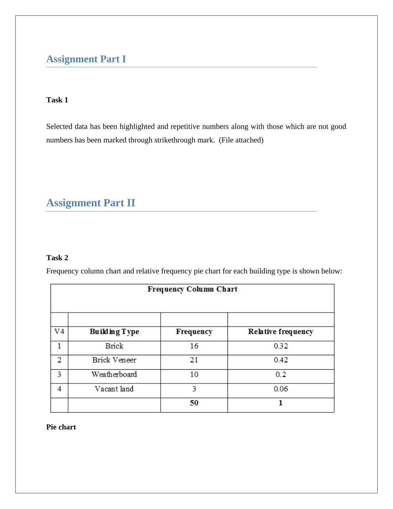
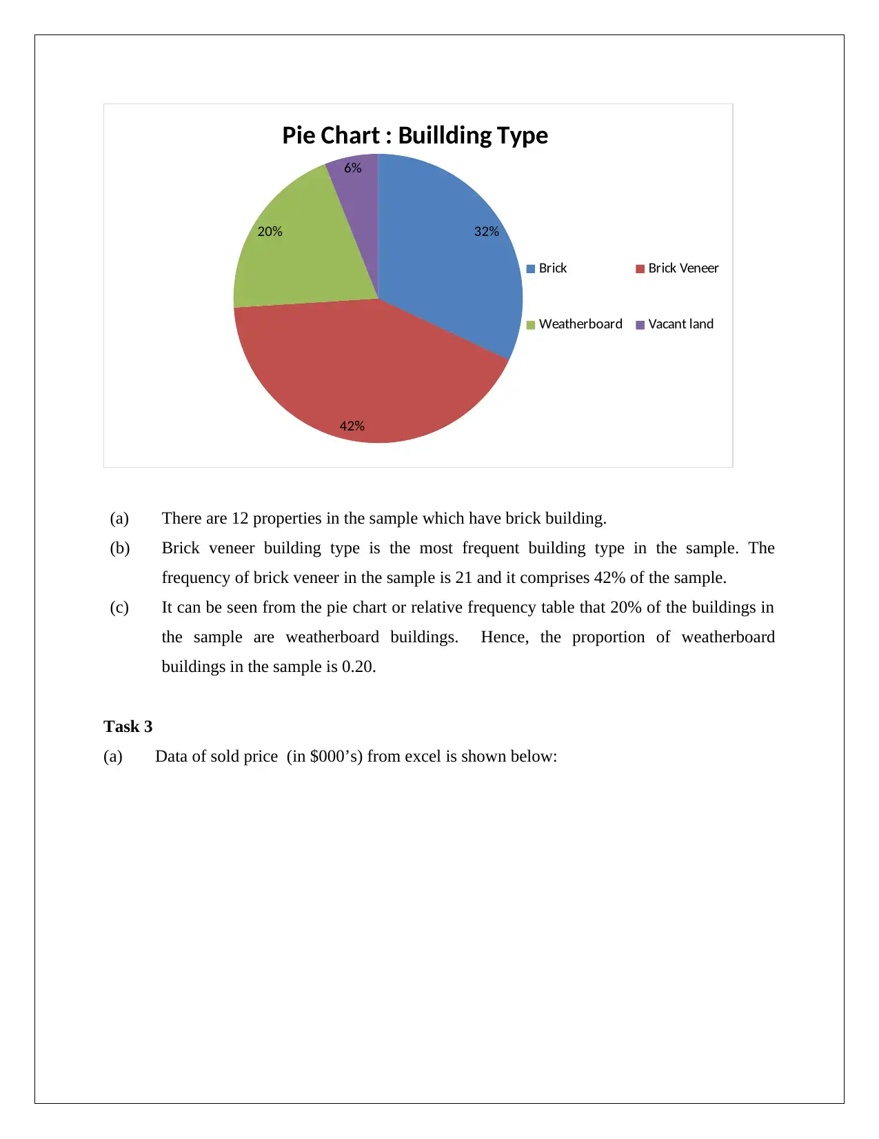
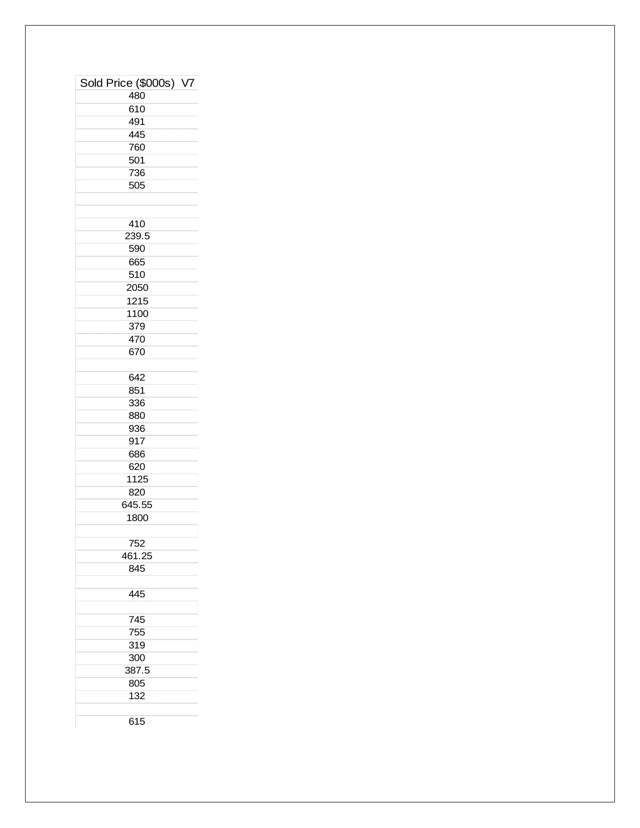
This Business Statistics assignment analyzes a dataset related to sold house prices. It includes tasks involving data cleaning, frequency distributions, and descriptive statistics, such as calculating percentiles, quartiles, and interquartile ranges. The assignment explores measures of central tendency and dispersion, determines the suitability of mean versus median, and assesses the normality of the data. It also calculates confidence intervals for both the mean sold price and the proportion of brick veneer properties. The analysis considers skewness, kurtosis, and the impact of outliers on the data distribution. The student also makes assumptions about the sold price population data and validates the findings.

Business Statistics
Assignment
STUDENT NUMBER (ID)
[Pick the date]

Assignment Part I
Task 1
Selected data has been highlighted and repetitive numbers along with those which are not good
numbers has been marked through strikethrough mark. (File attached)
Assignment Part II
Task 2
Frequency column chart and relative frequency pie chart for each building type is shown below:
Pie chart

32%
42%
20%
6%
Pie Chart : Buillding Type
Brick Brick Veneer
Weatherboard Vacant land
(a) There are 12 properties in the sample which have brick building.
(b) Brick veneer building type is the most frequent building type in the sample. The
frequency of brick veneer in the sample is 21 and it comprises 42% of the sample.
(c) It can be seen from the pie chart or relative frequency table that 20% of the buildings in
the sample are weatherboard buildings. Hence, the proportion of weatherboard
buildings in the sample is 0.20.
Task 3
(a) Data of sold price (in $000’s) from excel is shown below:

Sold Price ($000s) V7
480
610
491
445
760
501
736
505
410
239.5
590
665
510
2050
1215
1100
379
470
670
642
851
336
880
936
917
686
620
1125
820
645.55
1800
752
461.25
845
445
745
755
319
300
387.5
805
132
615

(b) The given percentile location formula 100
P
)1+n(=LP
(i) 70th Percentile
Here,
n=observations=43
P=Required percentile=70
Lp= ( n+ 1 ) P
100 = ( 43+ 1 ) 70
100 =30.8
Therefore, 70th Percentile would be the value of 31st term i.e. = $760, 000
(ii) The value of 1st and 3rd quartile
 1st quartile
Here,
n=observations=43
P=Required percentile=25
Lp= ( n+ 1 ) P
100 = ( 43+ 1 ) 25
100 =11
Therefore, 1st quartile would be the value of 11st term i.e. = $461,250.
 3rd quartile
Here,
n=observations=43
P=Required percentile=75

Lp= ( n+ 1 ) P
100 = ( 43+ 1 ) 75
100 =33
Therefore, 3rd quartile would be the value of 33st term i.e. = $820,000
(c) Value of 70 percentile indicates that about 70% of the sample houses sold prices are
lower than or same as the value of 70 percentile.. Further, the rest 30% of the sample
houses are having the sold price higher than $760, 000.
(d) Determination of Inter- Quartile Range of sold price
¿ $ 820,000−$ 461,250
¿ $ 358,750
 Inter-quartile range is considered to be a key measure of dispersion. This is because it
provides the estimation of the middle 50% of the total values in the provided dataset.
 IQR metric is more popular dispersion measure as compared with the range. This is because
range can be affected by the presence of outliers but there is not major effect of outliers on
inter- quartile range.
Task 4
(a) The summary statistics or descriptive statistics of variable sold price is shown below:

(b) Upper and lower inner fence limits is computed below:
 Upper limit inner fence
3 rd quartile=Q3=$ 820,000
Inter−quartile range=IQR=$ 358,750
IFUL=820,000+ ( 1.5∗358750 ) =$ 1358,125
 Lower limit inner fence
1 st quartile=Q1=$ 461,250
Inter−quartile range=IQR=$ 358,750
IFLL=461,250− ( 1.5∗358750 )=−$ 76,875

(C) The given cases and their description are shown below:
(i) As per the descriptive statistics and upper and lower inner fence limit, it can be said that
the most suitable measure of central tendency for the variable sold price of houses is
“median.”
The main reason behind this choice can be view with the fact that mean would not be the
suitable measure of central tendency because the presence of outliers in the rightwards
side would result distortion of mean and hence, it would not be a suitable measure.
(ii) As highlighted above that the most suitable measure of dispersion would be the “Inter-
quartile range.”
The reason behind the choice is that IQR is more about to determine the middle 50%
values among the total values and hence, it would not consider the higher values. Further,
the other measures of dispersion such as range and standard deviation would not be
suitable here.
Task 5
(a) Given set of data is not showing normal distribution because of the following reasons.
 In this case positive skew (+ 1.87) is present. Presence of skew is the indication of non-

normal distribution of data.
 Kurtosis (5.03), which is higher than 3. Value of kurtosis greater than 3 is the indication of
non-normal distribution of data.
 Measures of central tendency i.e. mean, mode and median are not same and hence, data is not
normally distributed.
(b) Assumption – Sold price population data - normally distributed
Values lie within 1.5 standard deviation of the given mean value i.e. between z=1.5∧z=−1.5 .
With the help of Standard normal table
P ( z<−1.5 )=0.0668∧P ( z <1.5 ) =0.9322
Now,
P (−1.5< z <1.5 )=0. 9322−0.0668=0.8664
Therefore, there are nearly 86.6% of total observations (i.e. 43) would lie within 1.5 standard
deviation of the given mean value.
Hence, number of values = 86.6% of 43 = 37 houses
(c) Value of mean = $ 689,460
Value of standard deviation = $365,020
Lower value = Mean – 1.5 standard deviation = 689460−1.5∗365020=$ 141,932.02
Upper value = Mean + 1.5 standard deviation = 689460+1.5∗365020=$ 1 ,236,988.906
Number of values within this range = 40
Number of values this case is higher than the number of values computed in part (b) and hence, it
statistically supports the findings of part (a) i.e. the sold price data is not normally distributed.
Task 6

(a) Descriptive statistics of variable sold price
(i) Point estimates (mean sold price) = $689460
(ii) Confidence interval ¿ mean ±Confidence level
Lower limit of 90% confidence interval = 689460−93630=$ 595,830
Upper limit of 90% confidence interval = 689460+93630=$ 783,090
(iii) Based on the confidence interval, it can be said with 90% confidence that mean sold price
of the houses ($) would fall within the range [595830 783090].
(b) It is apparent that the given mean value i.e. mean = $650,000 falls within the 90% confidence
interval range and therefore, it can be said that this confidence interval estimate is correct and
satisfactory.
Task 7

(a) Descriptive statistics for “brick veneer properties”
(i) Point estimates (mean of brick veneer properties) = 0.42
(ii) Confidence interval ¿ mean ±Confidence level
Lower limit of 99% confidence interval = 0.42−0.19=0.23
Upper limit of 99% confidence interval = 0.42+0.19=0.61
(b) 95% confidence interval estimation
If it is good normal distribution then t value would be taken into account. For 95% confidence
interval the t value is 1.96.
Hence,
Lower limit of 99% confidence interval = 0.42−1.96∗ √ 0.42 ( 1−0.42 )
50 =0.283
Upper limit of 99% confidence interval = 0.42+1.96∗
√ 0.42 ( 1−0.42 )
50 =0.556
Therefore, 95% confidence interval would be [0.283 0.556].

c) In part (b), the 95% confidence interval is obtained in comparison with part (a) where 99%
confidence interval is obtained. The probability associated with part (a) interval of finding the
mean is 99% which is higher than the corresponding probability in part (b) which is 95%. Owing
to the higher precision of interval in (a), it is more wider than the confidence interval obtained in
part (b) as it must account for greater aberrations in the mean value.