Business Statistics (MA/GA 508) Assignment - Part I & II Analysis

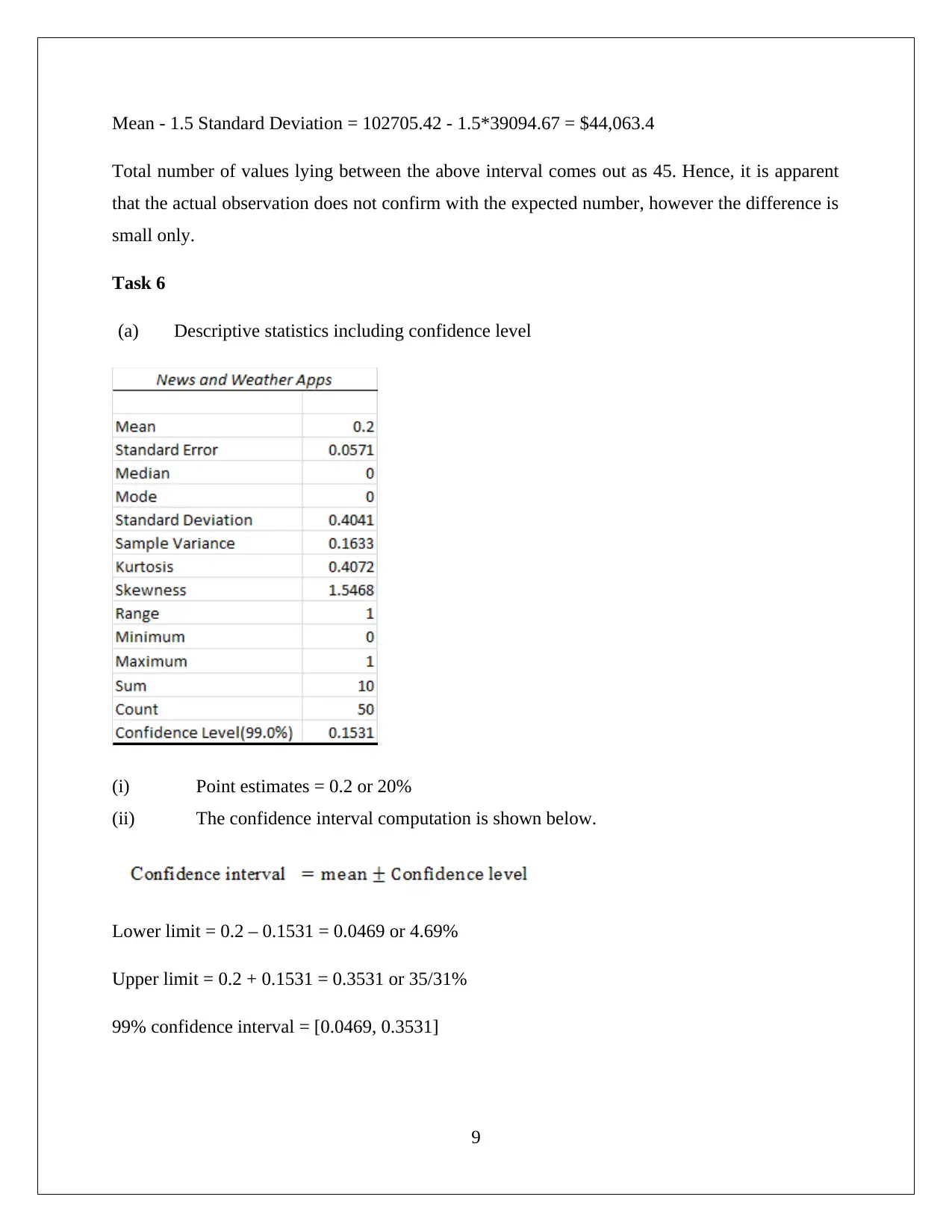
This document presents a comprehensive solution to a business statistics assignment, encompassing various statistical techniques and their applications. It begins with data selection and analysis, including frequency distributions and graphical summaries of entertainment content. The solution then delves into descriptive statistics, calculating percentiles, quartiles, and the interquartile range to analyze income data. The analysis extends to assessing the normality of income distribution and performing hypothesis testing related to the normal distribution. The assignment further explores confidence intervals and their interpretations, followed by a regression analysis to examine the relationship between age and smartphone usage for work. The solution includes detailed calculations, interpretations, and conclusions, providing a thorough understanding of statistical concepts and their practical applications in business contexts.

BUSINESS STATISTICS MA/GA 508
STUDENT ID
[Pick the date]

Assignment Part I
Task 1
The sample data of 50 observations has been determined by using random data sheet based on
the last three digits of student id i.e. (959). The main focus is to select the data between 001 and
300. The selected three digit data has been marked through strikethrough mark and the repetitive
number has been highlighted in the random data sheet pdf .
Assignment Part II
Task 2
The table represents the frequency table for the variable entertainment content.
1

(a) Frequency Column Chart
Music Video and
Movies News and
Weather Apps IM and Social
Network Apps Games eBooks Maps and
Navigation
Apps
0
2
4
6
8
10
12
14
16
18
FREQUENCY COLUMN CHART
ENTERTAINMENT CONTENT
Entertainment Content
Frequency
Relative frequency Pie Chart
2

Music ; 0.32
Video and Movies ; 0.04News and Weather
Apps ; 0.2
IM and Social
Network Apps ; 0.24
Games ; 0.16
eBooks ; 0.02 Maps and Navigation Apps ; 0.02
RELATIVE FREQUENCY PIE CHART
ENTERTAINMENT CONTENT
Graphical Summary
(a) The frequency of Music, Video and Movies entertainments is 18.
(b) “Music” entertainment type is showing maximum frequency with a frequency of 16.
(c) Proportion of entertainment type consisting of eBooks = 0.02 or 2%
Task 3
(a) Sorted data of annual income of the smart phone user ($) is shown below:
3

4

(b) Percentile location formula
100
P
)1+n(=LP
(i) 70th Percentile
n=Number of observations=50
P=Desired percentile=70
Lp= ( n+ 1 ) P
100
¿ ( 50+1 ) 70
100 =35.7
Hence, the 70th Percentile would be the corresponding value of 36st term = $99,398
(ii) The value of first and third quartile
 First quartile
n=Number of observations=50
P=Desired percentile=25
Lp= ( n+ 1 ) P
100 = ( 50+1 ) 25
100 =12.75
Hence, first quartile would be the corresponding value of 13st term = $94,600
 Third quartile
n=Number of observations=50
P=Desired percentile=75
Lp= ( n+ 1 ) P
100 = ( 50+1 ) 75
100 =38.25
5

Hence, 3rd quartile would be the corresponding value of 38st term = $99,650.
(c) The 70th percentile income level indicates that 70% of the sample users have an income
not exceeding $99,398.
(d) The Inter- Quartile Range (IQR)
IQR=$ 99,650−$ 94,600=$ 5,050
The above computation provides information that the middle 50% of the sample has the income
level range of $ 5,050 which is quite narrow. Hence, the dispersion in income level seems on the
lower side.
Task 4
(a) Descriptive statistics for variable “Income”
6

(b) Based on the above computation the value of upper and lower inner fence limits is given
below:
Upper limit inner fence is computation below:
Q3=$ 99,650
IQR=$ 5,050
IFUL=99,650+ ( 1.5∗5,050 ) =$ 107,225
Lower limit inner fence is computation below:
Q1=$ 94,600
IQR=$ 5,050
IFLL=$ 94,600− ( 1.5∗5050 ) =$ 87,025
(c) (i) The appropriate measure for central tendency would be median as the data has many
outliers especially on the higher side. This would tend to distort the mean and hence
taking median as the central tendency measure is recommended.
(ii) For capturing the dispersion, the IQR or interquartile range seems to be an
appropriate parameter as the standard deviation may not produce correct results owing to
the presence of outliers in the income data as some super rich are present in the data set.
7

(d) It is apparent that median is lower than the mean which may be attributed to the
presence of outliers on the higher end. Thus, usage of median has been recommended.
Further, the first quartile of income is $ 94,600 while the median (second quartile) is $
98,117.50. Further, the third quartile of the income level lies at $99.650. This clearly
highlights that the barring the outliers on the lower and higher end, the variation in
income level of smartphone users is quite low. Hence, the dispersion is largely
contributed by the presence of outliers, ignoring which the dispersion is quite minimal.
Task 5
(a) Three pieces of evidence are as highlighted below.
 For normal distribution, the skew should be zero whereas the given data has a high
amount of positive skew.
 There is non-coincidence of the measures of central tendency as the mean, median and
mode values are different. This is not permissible for a normal distribution.
 The kurtosis value is not equal to 3 which is another requirement for a normal
distribution.
Hence, in wake of the above discussion, it would be fair to conclude that the income distribution
is not normal.
b) P (Z<-1.5) = 0.0668 (From z table)
P (Z<1.5) = 0.9332 (From z table)
Hence, P(-1.5<Z<1.5) = 0.9332 -0.0668 = 0.8664 or 86.64%
Thus, given the sample size of 60, expected number of values expected to fall in the given
interval = (86.64/100)*50 = 43
c) Mean + 1.5 Standard Deviation = 102705.42 + 1.5*39094.67 = $161,347.43
8

Mean - 1.5 Standard Deviation = 102705.42 - 1.5*39094.67 = $44,063.4
Total number of values lying between the above interval comes out as 45. Hence, it is apparent
that the actual observation does not confirm with the expected number, however the difference is
small only.
Task 6
(a) Descriptive statistics including confidence level
(i) Point estimates = 0.2 or 20%
(ii) The confidence interval computation is shown below.
Lower limit = 0.2 – 0.1531 = 0.0469 or 4.69%
Upper limit = 0.2 + 0.1531 = 0.3531 or 35/31%
99% confidence interval = [0.0469, 0.3531]
9

b) 95% confidence z value = 1.959
Lower limit = 0.2 + 1.959*0.0571 = 0.0881 or 8.81%
Upper limit = 0.2 + 1.959*0.0571 = 0.3119 or 31.19%
Hence, the 95% confidence interval is [0.0881, 0.3119]
c) The 99% confidence interval is wider in comparison to the 95% confidence interval which is
on expected lines since the precision is more for a 99% confidence interval in comparison for a
95% confidence interval. As a result, the 99% confidence interval needs to be wider so as to
cover possibilities which have lesser probability of happening.
Task 7
a) The estimated regression equation is as stated below.
Percent for work = -6.855+0.608Age
b) The requisite hypotheses are stated below.
Ho: βAge = 0
H1: βAge ≠ 0
c) Based on the ANOVA output, it is apparent that F statistic comes out as 43.25 while the
corresponding p value comes out as zero. Assuming a significance level of 5%, it is apparent
that p value is lower than the significance level. Hence, sufficient evidence for null hypothesis
rejection is available which indicates that the regression model is sufficient as slope cannot be
assumed to be zero.
d) The intercept coefficient highlights the percent of phone usage for work when age is zero.
Clearly, this does not make sense as a person who has the age zero cannot use a smartphone.
Also, the percentage value of time cannot be negative.
10

e) The slope coefficient implies that as the age increases by one year, the percentage usage of
phone for work purpose increases by 0.608%. A decrease of the same percentage would be
observed if there is a decrease of age by one year.
f) The coefficient of determination or R2 has a value of 0.1267. This implies that only 12.67% of
the changes in dependent variable (i.e. percent of work) can be explained by corresponding
changes in the independent variable (i.e. age). This implies that there are other variables on
which the percent of work would depend which need to be built into the given regression
model.
11