CIS116-6 Wireless Embedded Systems: Assignment Part-I Control Solution

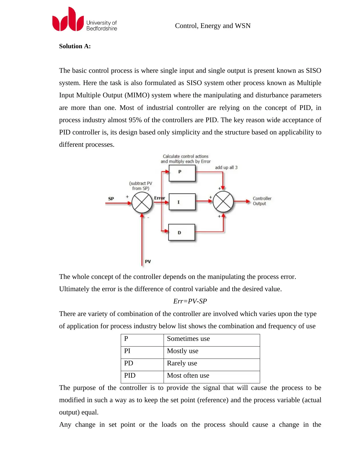
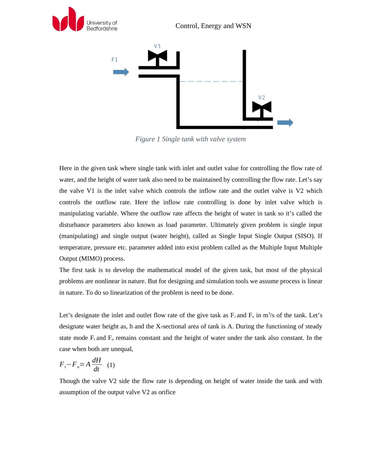
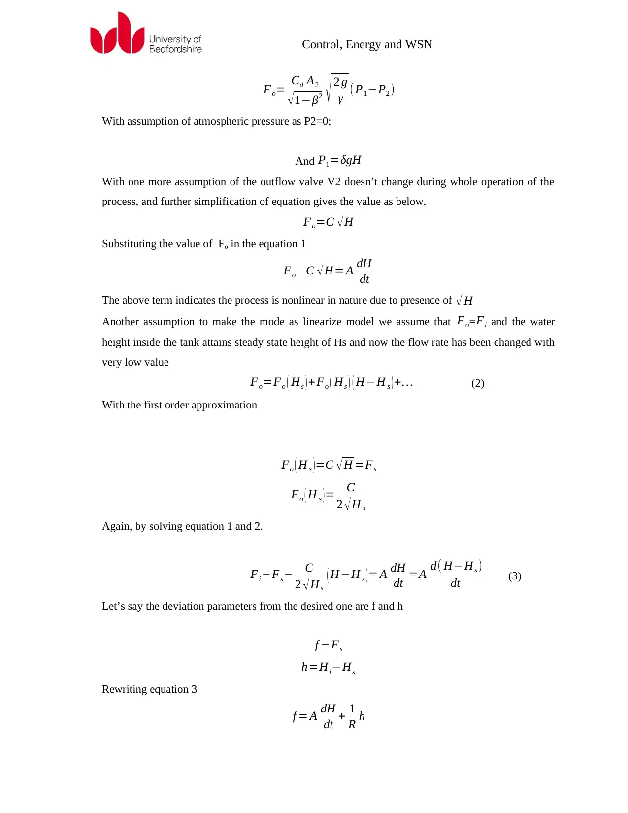
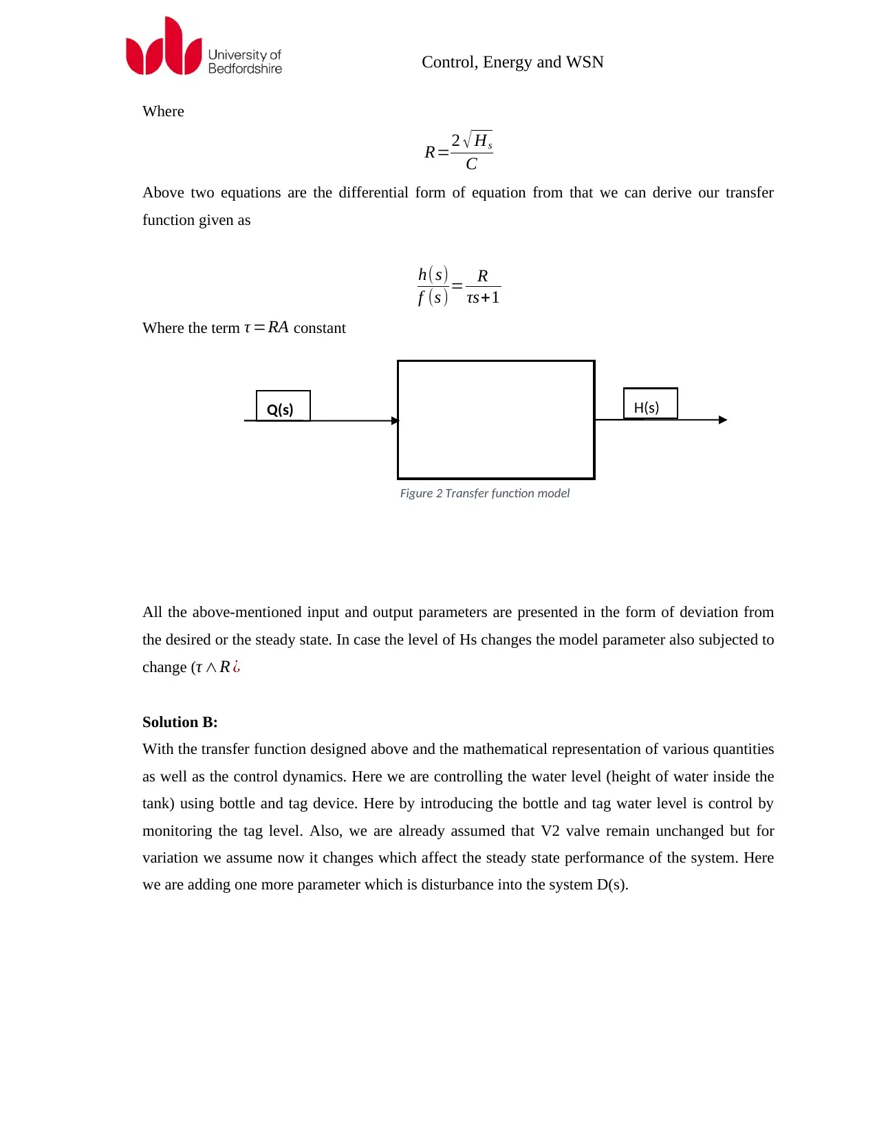
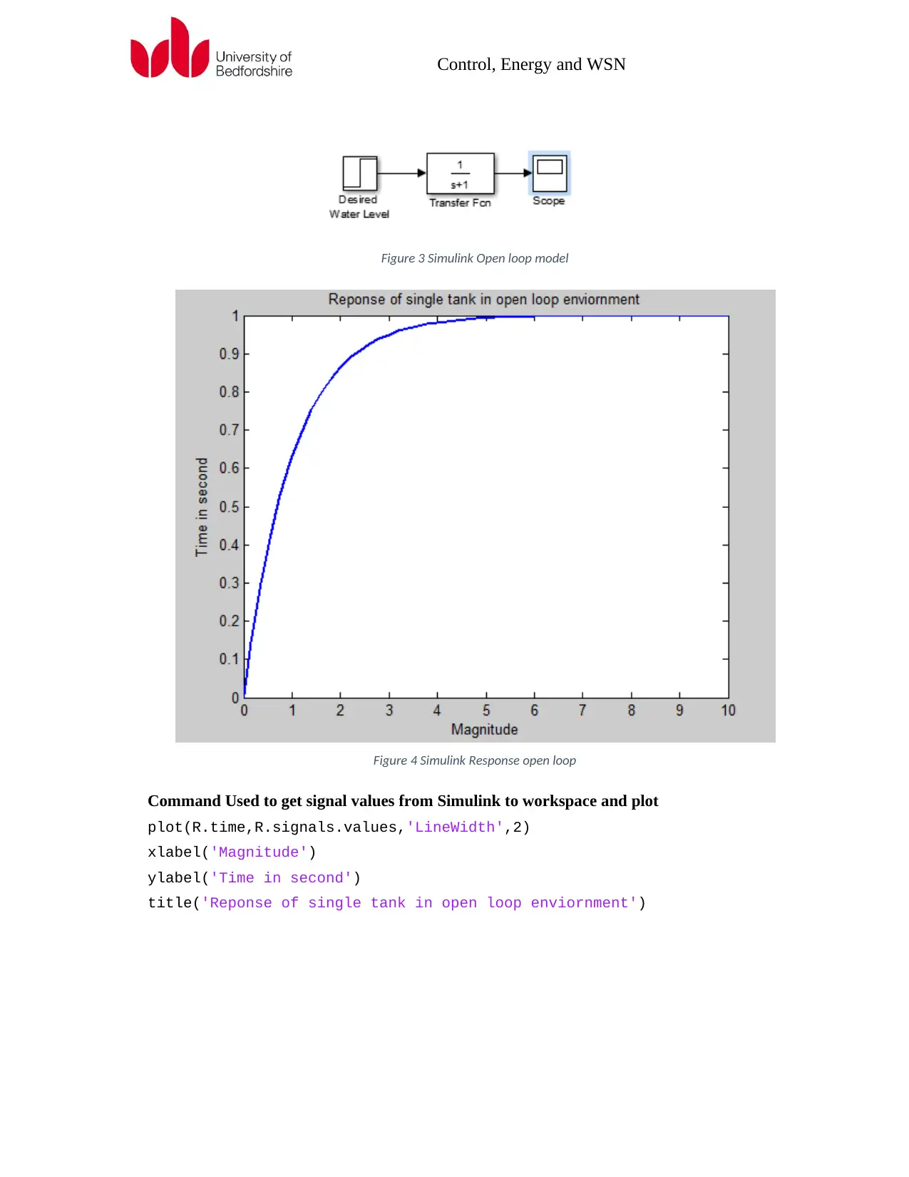
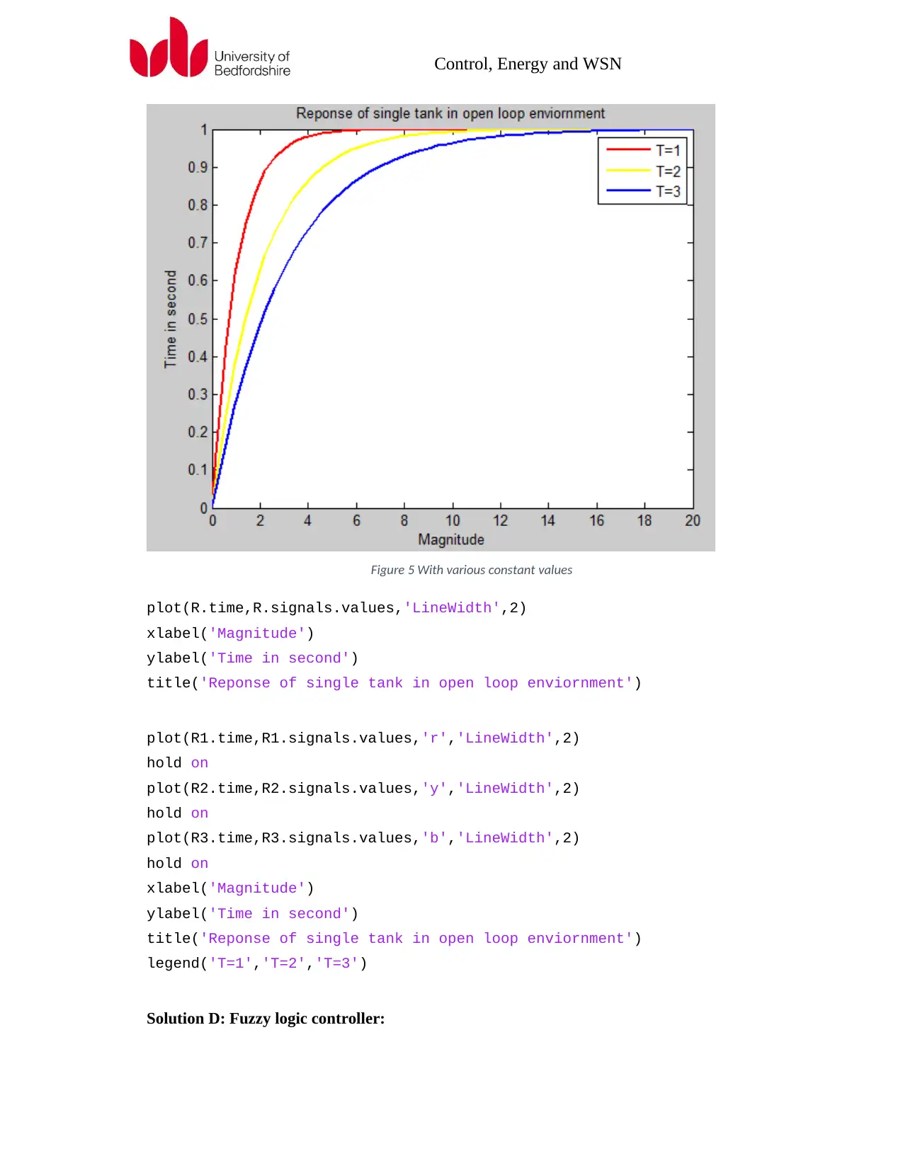
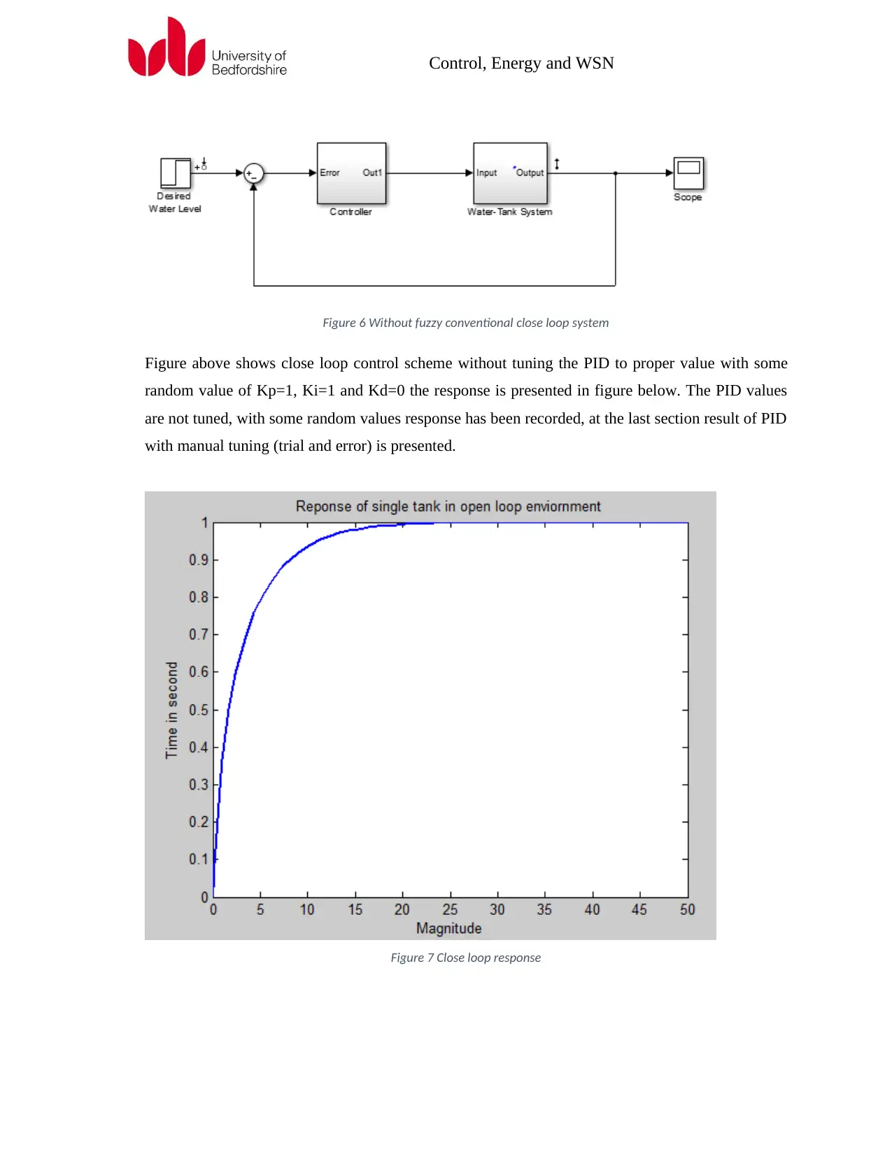
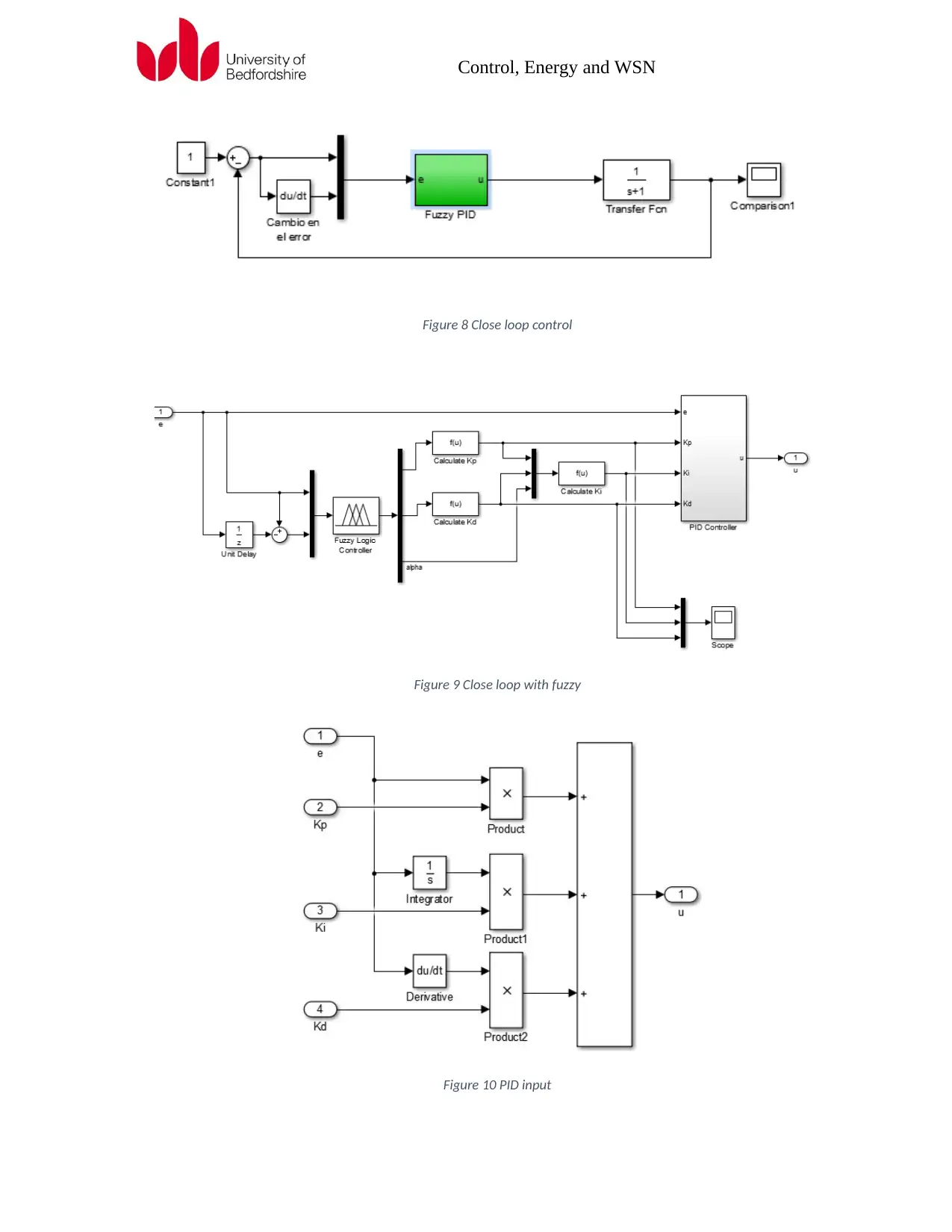
This assignment solution for CIS116 Wireless Embedded Systems addresses the control of a single-tank system. The solution begins with an overview of control processes, including SISO and MIMO systems, and the application of PID controllers. It then details the design of a single-tank system with inlet and outlet valves, deriving the mathematical model and transfer function for the system. The solution incorporates the use of a bottle and tag system for water level control. The assignment further develops a fuzzy logic controller using MATLAB Simulink and integrates it into a closed-loop control system. The performance of the closed-loop system is evaluated, with analysis of rise time, settling time, and stability. Open loop and closed loop simulations are presented, along with the analysis of the system with and without fuzzy logic controller, comparing the performance of different tuning methods. The report also provides MATLAB code and simulation results to validate the findings. The assignment's primary focus is on analyzing control systems, designing controllers, and evaluating system performance through simulation and mathematical modeling.

CIS116-6 Wireless Embedded Systems
Assignment Part-I

Control, Energy and WSN
Solution A:
The basic control process is where single input and single output is present known as SISO
system. Here the task is also formulated as SISO system other process known as Multiple
Input Multiple Output (MIMO) system where the manipulating and disturbance parameters
are more than one. Most of industrial controller are relying on the concept of PID, in
process industry almost 95% of the controllers are PID. The key reason wide acceptance of
PID controller is, its design based only simplicity and the structure based on applicability to
different processes.
The whole concept of the controller depends on the manipulating the process error.
Ultimately the error is the difference of control variable and the desired value.
Err=PV-SP
There are variety of combination of the controller are involved which varies upon the type
of application for process industry below list shows the combination and frequency of use
P Sometimes use
PI Mostly use
PD Rarely use
PID Most often use
The purpose of the controller is to provide the signal that will cause the process to be
modified in such a way as to keep the set point (reference) and the process variable (actual
output) equal.
Any change in set point or the loads on the process should cause a change in the

Control, Energy and WSN
controller’s output to assure that the PV tracks SP.
Types of analog controller
1. simple ON/OFF controller (cycling or chatter)
2. proportional controller
3. Proportional Integral controller
4. PID controller (good transient & Steady state control)
The most important block in an analog controller is the ERROR AMPLIFIER
Proportional:
P controller widely use in the first order system to stabilize the unstable process. It helps in
decreasing the steady state error. with increase in gain of the system the steady state error
reduces. With high value of P it gives smaller amplitude and phase margin also reduce
noise signal
Drawback of proportional controller
The error can’t be eliminated completely. To reduces the error, the controller must raise its
output. But to raise its output, the controller must have some error. This residual error can
be reduced by increasing the gain but too much gain will cause the system to oscillate.
Derivative:
Integral control doesn’t provide capability to predict the future error of the system, so the
response is very normal even after the changes occur in set point (reference). The use of
derivative controller can avoid such issues by predicting the future response of the error
signal. The output of the plant or process dependent on the rate of change of the error signal
with time and whole things multiplied by the D-constant.
Integral:
To eliminate the residual system error, the controller’s response must be changed. In
proportional controller the output was proportional to the system error.
PID:

Control, Energy and WSN
PID controller helps in optimal control with no steady state error, zero oscillations, good
stability and fast response. With PI controller use of Derivative helps in eliminate the
overshoot and oscillations of the system of the output response. It also having advantage of
can be implemented for higher order system.
Tuning of PID controller:
The dynamics of process need to be controlled with the use of PID controller, each term of
PID controller have their own characteristics and properties. Without tuning PID controller
the response of the system may cause very high deviation and instability of the system.
Various tuning methods are used in field of control engineering namely few are trial and
error method, process reaction curve, Ziegler Nichols method and modern meta heuristic
based tuning. One of the best suitable method is fuzzy controller.
Trial and Error method:
The open loop response first recorded based on that PID controller is installed after that
tuning is the important process. In this method the parameter of PID are set to zero and
increase the value of Kp till the response attain oscillations. After oscillations occurs
Integral value also adjusted and finally Derivative to obtain the quick response.
Process Reaction Curve Method:
Ultimately, it’s the open loop method. The input is step unit signal and the response of the
system is recorded. Than from the slope of the curve we can find the value of P,I and D
parameters.
Normally the process in engineering may contains number of input and output variables.
Though only one or two of the parameters are needed to control the whole process of the
plant model. Such controlling parameters are known as manipulating variable, and other
may be uncontrollable which are known as the disturbance parameters. Generally, the
controller has the feedback system where output of system is taken and compared with the
desired or set value if any deviation found in the comparison, corrective action is taken
correspondingly.

Control, Energy and WSN
Figure 1 Single tank with valve system
Here in the given task where single tank with inlet and outlet value for controlling the flow rate of
water, and the height of water tank also need to be maintained by controlling the flow rate. Let’s say
the valve V1 is the inlet valve which controls the inflow rate and the outlet valve is V2 which
controls the outflow rate. Here the inflow rate controlling is done by inlet valve which is
manipulating variable. Where the outflow rate affects the height of water in tank so it’s called the
disturbance parameters also known as load parameter. Ultimately given problem is single input
(manipulating) and single output (water height), called as Single Input Single Output (SISO). If
temperature, pressure etc. parameter added into exist problem called as the Multiple Input Multiple
Output (MIMO) process.
The first task is to develop the mathematical model of the given task, but most of the physical
problems are nonlinear in nature. But for designing and simulation tools we assume process is linear
in nature. To do so linearization of the problem is need to be done.
Let’s designate the inlet and outlet flow rate of the give task as Fi and Fo in m3/s of the tank. Let’s
designate water height as, h and the X-sectional area of tank is A. During the functioning of steady
state mode Fi and Fo remains constant and the height of water under the tank also constant. In the
case when both are unequal,
Fi−Fo= A dH
dt (1)
Though the valve V2 side the flow rate is depending on height of water inside the tank and with
assumption of the output valve V2 as orifice

Control, Energy and WSN
Fo= Cd A2
√1−β2 √ 2 g
γ (P1−P2 )
With assumption of atmospheric pressure as P2=0;
And P1=δgH
With one more assumption of the outflow valve V2 doesn’t change during whole operation of the
process, and further simplification of equation gives the value as below,
Fo=C √ H
Substituting the value of Fo in the equation 1
Fo−C √H= A dH
dt
The above term indicates the process is nonlinear in nature due to presence of √ H
Another assumption to make the mode as linearize model we assume that Fo= Fi and the water
height inside the tank attains steady state height of Hs and now the flow rate has been changed with
very low value
Fo=Fo ( Hs ) +Fo ( Hs ) ( H−H s ) +… (2)
With the first order approximation
Fo ( H s )=C √ H =Fs
Fo ( H s ) = C
2 √ H s
Again, by solving equation 1 and 2.
Fi−Fs− C
2 √ Hs
( H−H s ) = A dH
dt =A d( H−Hs )
dt (3)
Let’s say the deviation parameters from the desired one are f and h
f −Fs
h=Hi−Hs
Rewriting equation 3
f = A dH
dt + 1
R h

Control, Energy and WSN
Where
R=2 √ Hs
C
Above two equations are the differential form of equation from that we can derive our transfer
function given as
h(s)
f (s ) = R
τs+1
Where the term τ =RA constant
All the above-mentioned input and output parameters are presented in the form of deviation from
the desired or the steady state. In case the level of Hs changes the model parameter also subjected to
change (τ ∧R ¿
Solution B:
With the transfer function designed above and the mathematical representation of various quantities
as well as the control dynamics. Here we are controlling the water level (height of water inside the
tank) using bottle and tag device. Here by introducing the bottle and tag water level is control by
monitoring the tag level. Also, we are already assumed that V2 valve remain unchanged but for
variation we assume now it changes which affect the steady state performance of the system. Here
we are adding one more parameter which is disturbance into the system D(s).
Q(s) H(s)
Figure 2 Transfer function model

Control, Energy and WSN
If the system having the error signal ¿ Ees
Bottle and tag controlling of valve V1 ¿ Bv
Gs = R
τS+1
The controlling parameter is ¿ Ees Bv
Cs
Rs
= Bv R
τS +1
If R and Bv are constant, another constant K can be defined and equation can be rewrite as
below
Cs
Rs
= K
τS +1
Cs= Rs∗1
τS+1
Solution C:
At the initial modeling stage in MATLAB Simulink first the open loop model of the system has
been analyzed with the given transfer function. Below figure illustrate simple open loop transfer
function without any feedback and disturbance.

Control, Energy and WSN
Figure 3 Simulink Open loop model
Figure 4 Simulink Response open loop
Command Used to get signal values from Simulink to workspace and plot
plot(R.time,R.signals.values,'LineWidth',2)
xlabel('Magnitude')
ylabel('Time in second')
title('Reponse of single tank in open loop enviornment')

Control, Energy and WSN
Figure 5 With various constant values
plot(R.time,R.signals.values,'LineWidth',2)
xlabel('Magnitude')
ylabel('Time in second')
title('Reponse of single tank in open loop enviornment')
plot(R1.time,R1.signals.values,'r','LineWidth',2)
hold on
plot(R2.time,R2.signals.values,'y','LineWidth',2)
hold on
plot(R3.time,R3.signals.values,'b','LineWidth',2)
hold on
xlabel('Magnitude')
ylabel('Time in second')
title('Reponse of single tank in open loop enviornment')
legend('T=1','T=2','T=3')
Solution D: Fuzzy logic controller:

Control, Energy and WSN
Figure 6 Without fuzzy conventional close loop system
Figure above shows close loop control scheme without tuning the PID to proper value with some
random value of Kp=1, Ki=1 and Kd=0 the response is presented in figure below. The PID values
are not tuned, with some random values response has been recorded, at the last section result of PID
with manual tuning (trial and error) is presented.
Figure 7 Close loop response

Control, Energy and WSN
Figure 8 Close loop control
Figure 9 Close loop with fuzzy
Figure 10 PID input