Financial Analysis and Investment Appraisal Report - University
VerifiedAdded on 2021/04/24
|23
|2433
|21
Report
AI Summary
This report provides a comprehensive analysis of financial decision-making for a business, evaluating various investment appraisal methods and their implications. It begins with a decision analysis for Dream Catcher, comparing international and domestic expansion with a no-change scenario, and recommends international expansion based on profit projections. The report then assesses mortgage alternatives for Kyle Dier, comparing lenders like HSBC-UK, Virgin Money, and Chesler Building Society, ultimately recommending HSBC for its lower monthly payments. Next, it reviews profitable models for a table product line, using linear regression across three scenarios to maximize profit. Finally, the report demonstrates investment appraisal methods such as net present value, internal rate of return, accounting rate of return, and payback period, analyzing investment projects for Pierce Plc, and recommending investment in product Y based on payback period and IRR criteria. The report also includes an analysis of expected and actual exam scores, covering topics in Quantitative Methods and Accounting.
Running head: BUSINESS
Business
Name of the Student
Name of the University
Author Note
Business
Name of the Student
Name of the University
Author Note
Paraphrase This Document
Need a fresh take? Get an instant paraphrase of this document with our AI Paraphraser
1
BUSINESS
Table of Contents
Question 1:.................................................................................................................................3
Introduction:...........................................................................................................................3
Requirement a).......................................................................................................................3
Requirement b).......................................................................................................................4
Conclusion:............................................................................................................................4
Question 2:.................................................................................................................................5
Introduction:...........................................................................................................................5
Requirement a).......................................................................................................................5
Requirement b).......................................................................................................................5
Requirement c).......................................................................................................................9
Requirement d).....................................................................................................................12
Conclusion:..........................................................................................................................13
Question 3:...............................................................................................................................13
Introduction:.........................................................................................................................13
Discussion:...........................................................................................................................13
Conclusion:..........................................................................................................................17
Question 4:...............................................................................................................................18
Introduction:.........................................................................................................................18
Requirement a).....................................................................................................................18
2
BUSINESS
Requirement b).....................................................................................................................20
Requirement c).....................................................................................................................21
Conclusion:..........................................................................................................................21
Question 5:...............................................................................................................................22
Requirement a).....................................................................................................................22
Requirement b).....................................................................................................................23
Requirement c).....................................................................................................................24
References list:.........................................................................................................................26
⊘ This is a preview!⊘
Do you want full access?
Subscribe today to unlock all pages.
Trusted by 1+ million students worldwide
3
BUSINESS
Question 1:
Introduction:
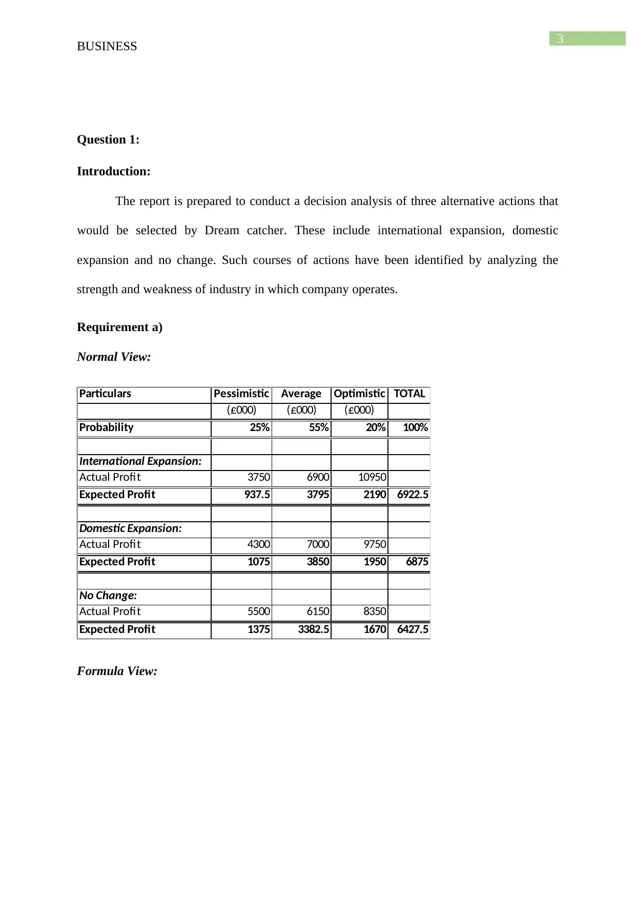
The report is prepared to conduct a decision analysis of three alternative actions that
would be selected by Dream catcher. These include international expansion, domestic
expansion and no change. Such courses of actions have been identified by analyzing the
strength and weakness of industry in which company operates.
Requirement a)
Normal View:
Particulars Pessimistic Average Optimistic TOTAL
(£000) (£000) (£000)
Probability 25% 55% 20% 100%
International Expansion:
Actual Profit 3750 6900 10950
Expected Profit 937.5 3795 2190 6922.5
Domestic Expansion:
Actual Profit 4300 7000 9750
Expected Profit 1075 3850 1950 6875
No Change:
Actual Profit 5500 6150 8350
Expected Profit 1375 3382.5 1670 6427.5
Formula View:
BUSINESS
Question 1:
Introduction:
The report is prepared to conduct a decision analysis of three alternative actions that
would be selected by Dream catcher. These include international expansion, domestic
expansion and no change. Such courses of actions have been identified by analyzing the
strength and weakness of industry in which company operates.
Requirement a)
Normal View:
Particulars Pessimistic Average Optimistic TOTAL
(£000) (£000) (£000)
Probability 25% 55% 20% 100%
International Expansion:
Actual Profit 3750 6900 10950
Expected Profit 937.5 3795 2190 6922.5
Domestic Expansion:
Actual Profit 4300 7000 9750
Expected Profit 1075 3850 1950 6875
No Change:
Actual Profit 5500 6150 8350
Expected Profit 1375 3382.5 1670 6427.5
Formula View:
Paraphrase This Document
Need a fresh take? Get an instant paraphrase of this document with our AI Paraphraser
4
BUSINESS
Particulars Pessimistic Average Optimistic TOTAL
(£000) =B4 =C4
Probability 0.25 0.55 0.2 =SUM(B5:D5)
International Expansion:
Actual Profit 3750 6900 10950
Expected Profit =$B$5*B8 =$C$5*C8 =$D$5*D8 =SUM(B9:D9)
Domestic Expansion:
Actual Profit 4300 7000 9750
Expected Profit =$B$5*B12 =$C$5*C12 =$D$5*D12 =SUM(B13:D13)
No Change:
Actual Profit 5500 6150 8350
Expected Profit =$B$5*B16 =$C$5*C16 =$D$5*D16 =SUM(B17:D17)
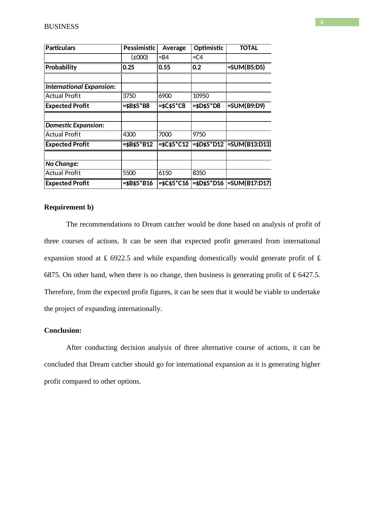
Requirement b)
The recommendations to Dream catcher would be done based on analysis of profit of
three courses of actions. It can be seen that expected profit generated from international
expansion stood at ₤ 6922.5 and while expanding domestically would generate profit of ₤
6875. On other hand, when there is no change, then business is generating profit of ₤ 6427.5.
Therefore, from the expected profit figures, it can be seen that it would be viable to undertake
the project of expanding internationally.
Conclusion:
After conducting decision analysis of three alternative course of actions, it can be
concluded that Dream catcher should go for international expansion as it is generating higher
profit compared to other options.
BUSINESS
Particulars Pessimistic Average Optimistic TOTAL
(£000) =B4 =C4
Probability 0.25 0.55 0.2 =SUM(B5:D5)
International Expansion:
Actual Profit 3750 6900 10950
Expected Profit =$B$5*B8 =$C$5*C8 =$D$5*D8 =SUM(B9:D9)
Domestic Expansion:
Actual Profit 4300 7000 9750
Expected Profit =$B$5*B12 =$C$5*C12 =$D$5*D12 =SUM(B13:D13)
No Change:
Actual Profit 5500 6150 8350
Expected Profit =$B$5*B16 =$C$5*C16 =$D$5*D16 =SUM(B17:D17)
Requirement b)
The recommendations to Dream catcher would be done based on analysis of profit of
three courses of actions. It can be seen that expected profit generated from international
expansion stood at ₤ 6922.5 and while expanding domestically would generate profit of ₤
6875. On other hand, when there is no change, then business is generating profit of ₤ 6427.5.
Therefore, from the expected profit figures, it can be seen that it would be viable to undertake
the project of expanding internationally.
Conclusion:
After conducting decision analysis of three alternative course of actions, it can be
concluded that Dream catcher should go for international expansion as it is generating higher
profit compared to other options.
5
BUSINESS
Question 2:
Introduction:
The report is prepared to ascertain the lenders for financing two possible properties
that Kyle Dier is seeking to buy. Mortgage alternatives are selected by determining applicable
interest rates and respective terms. Decision is also taken by considering several other factors.
Requirement a)
Three lenders that Kyle could borrow money for buying a one bedroom flat or a three-
bedroom house outside the town are ascertained. Such vendors include HSBC-UK, Virgin
money and Chesler building society. HSBC is one of the largest financial and banking service
organizations based in London. Virgin money is a provider of financial services that offers a
wide range of investment and savings product. Chesler building society is another financial
institution that offers financing and banking services.
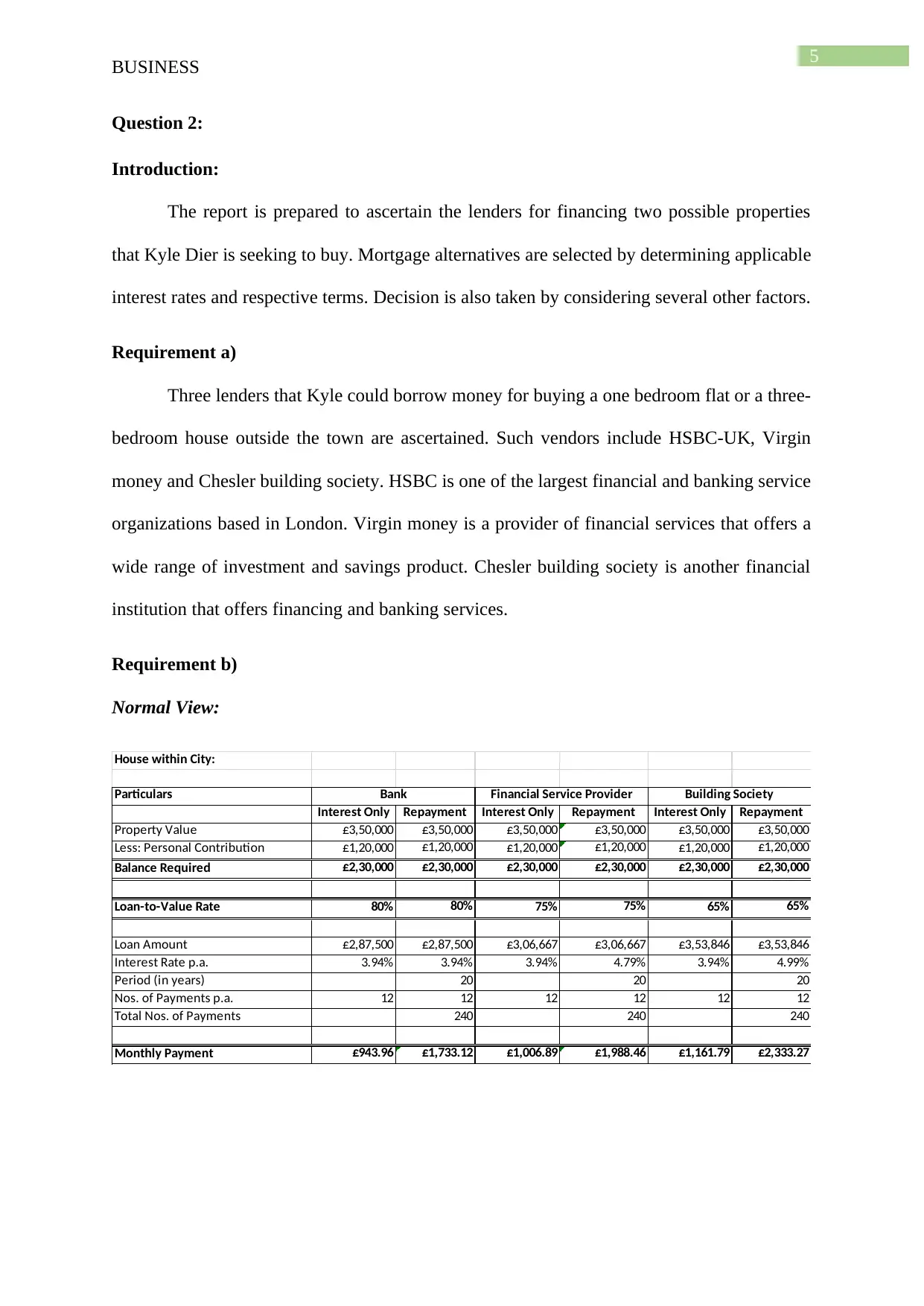
Requirement b)
Normal View:
House within City:
Particulars
Interest Only Repayment Interest Only Repayment Interest Only Repayment
Property Value £3,50,000 £3,50,000 £3,50,000 £3,50,000 £3,50,000 £3,50,000
Less: Personal Contribution £1,20,000 £1,20,000 £1,20,000 £1,20,000 £1,20,000 £1,20,000
Balance Required £2,30,000 £2,30,000 £2,30,000 £2,30,000 £2,30,000 £2,30,000
Loan-to-Value Rate 80% 80% 75% 75% 65% 65%
Loan Amount £2,87,500 £2,87,500 £3,06,667 £3,06,667 £3,53,846 £3,53,846
Interest Rate p.a. 3.94% 3.94% 3.94% 4.79% 3.94% 4.99%
Period (in years) 20 20 20
Nos. of Payments p.a. 12 12 12 12 12 12
Total Nos. of Payments 240 240 240
Monthly Payment £943.96 £1,733.12 £1,006.89 £1,988.46 £1,161.79 £2,333.27
Bank Financial Service Provider Building Society
BUSINESS
Question 2:
Introduction:
The report is prepared to ascertain the lenders for financing two possible properties
that Kyle Dier is seeking to buy. Mortgage alternatives are selected by determining applicable
interest rates and respective terms. Decision is also taken by considering several other factors.
Requirement a)
Three lenders that Kyle could borrow money for buying a one bedroom flat or a three-
bedroom house outside the town are ascertained. Such vendors include HSBC-UK, Virgin
money and Chesler building society. HSBC is one of the largest financial and banking service
organizations based in London. Virgin money is a provider of financial services that offers a
wide range of investment and savings product. Chesler building society is another financial
institution that offers financing and banking services.
Requirement b)
Normal View:
House within City:
Particulars
Interest Only Repayment Interest Only Repayment Interest Only Repayment
Property Value £3,50,000 £3,50,000 £3,50,000 £3,50,000 £3,50,000 £3,50,000
Less: Personal Contribution £1,20,000 £1,20,000 £1,20,000 £1,20,000 £1,20,000 £1,20,000
Balance Required £2,30,000 £2,30,000 £2,30,000 £2,30,000 £2,30,000 £2,30,000
Loan-to-Value Rate 80% 80% 75% 75% 65% 65%
Loan Amount £2,87,500 £2,87,500 £3,06,667 £3,06,667 £3,53,846 £3,53,846
Interest Rate p.a. 3.94% 3.94% 3.94% 4.79% 3.94% 4.99%
Period (in years) 20 20 20
Nos. of Payments p.a. 12 12 12 12 12 12
Total Nos. of Payments 240 240 240
Monthly Payment £943.96 £1,733.12 £1,006.89 £1,988.46 £1,161.79 £2,333.27
Bank Financial Service Provider Building Society
⊘ This is a preview!⊘
Do you want full access?
Subscribe today to unlock all pages.
Trusted by 1+ million students worldwide
6
BUSINESS
House Outside City:
Particulars
Interest Only Repayment Interest Only Repayment Interest Only Repayment
Property Value £5,00,000 £5,00,000 £5,00,000 £5,00,000 £5,00,000 £5,00,000
Less: Personal Contribution £1,20,000 £1,20,000 £1,20,000 £1,20,000 £1,20,000 £1,20,000
Balance Required £3,80,000 £3,80,000 £3,80,000 £3,80,000 £3,80,000 £3,80,000
Loan-to-Value Rate 80% 80% 75% 75% 65% 65%
Loan Amount £4,75,000 £4,75,000 £5,06,667 £5,06,667 £5,84,615 £5,84,615
Interest Rate p.a. 3.94% 3.94% 3.94% 4.79% 3.94% 4.99%
Period (in years) 20 20 20
Nos. of Payments p.a. 12 12 12 12 12 12
Total Nos. of Payments 240 240 240
Monthly Repayment £1,559.58 £2,863.41 £1,663.56 £3,285.28 £1,919.49 £3,854.97
Bank Financial Service Provider Building Society
Formula View:
House within City:
Particulars
Interest Only Repayment Interest Only Repayment Interest Only Repayment
Property Value =C5 350000 =E5 =C5 =G5 =E5
Less: Personal Contribution =C6 120000 =E6 =C6 =G6 =E6
Balance Required =B5-B6 =C5-C6 =D5-D6 =E5-E6 =F5-F6 =G5-G6
Loan-to-Value Rate =C9 0.8 =E9 0.75 =G9 0.65
Loan Amount =B7/B9 =C7/C9 =D7/D9 =E7/E9 =F7/F9 =G7/G9
Interest Rate p.a. 0.0394 0.0394 0.0394 0.0479 0.0394 0.0499
Period (in years) 20 =C13 =E13
Nos. of Payments p.a. 12 12 12 =C14 12 =E14
Total Nos. of Payments =C13*C14 =E13*E14 =G13*G14
Monthly Payment =B11*(B12/B14) =PMT((C12/C14),C15,-C11,0) =D11*(D12/D14) =PMT((E12/E14),E15,-E11,0) =F11*(F12/F14) =PMT((G12/G14),G15,-G11,0)
Bank Financial Service Provider Building Society
House Outside City:
Particulars
Interest Only Repayment Interest Only Repayment Interest Only Repayment
Property Value =L5 500000 =N5 =L5 =P5 =N5
Less: Personal Contribution =L6 120000 =N6 =L6 =P6 =N6
Balance Required =K5-K6 =L5-L6 =M5-M6 =N5-N6 =O5-O6 =P5-P6
Loan-to-Value Rate =L9 0.8 =N9 0.75 =P9 0.65
Loan Amount =K7/K9 =L7/L9 =M7/M9 =N7/N9 =O7/O9 =P7/P9
Interest Rate p.a. 0.0394 0.0394 0.0394 0.0479 0.0394 0.0499
Period (in years) 20 =L13 =N13
Nos. of Payments p.a. 12 12 12 =L14 12 =N14
Total Nos. of Payments =L13*L14 =N13*N14 =P13*P14
Monthly Repayment =K11*(K12/K14) =PMT((L12/L14),L15,-L11,0) =M11*(M12/M14) =PMT((N12/N14),N15,-N11,0) =O11*(O12/O14) =PMT((P12/P14),P15,-P11,0)
Bank Financial Service Provider Building Society
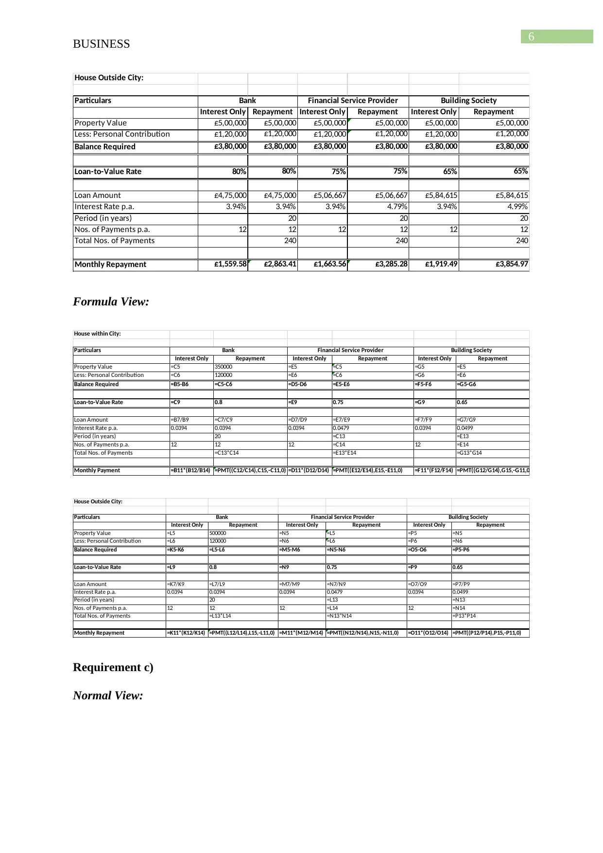
Requirement c)
Normal View:
BUSINESS
House Outside City:
Particulars
Interest Only Repayment Interest Only Repayment Interest Only Repayment
Property Value £5,00,000 £5,00,000 £5,00,000 £5,00,000 £5,00,000 £5,00,000
Less: Personal Contribution £1,20,000 £1,20,000 £1,20,000 £1,20,000 £1,20,000 £1,20,000
Balance Required £3,80,000 £3,80,000 £3,80,000 £3,80,000 £3,80,000 £3,80,000
Loan-to-Value Rate 80% 80% 75% 75% 65% 65%
Loan Amount £4,75,000 £4,75,000 £5,06,667 £5,06,667 £5,84,615 £5,84,615
Interest Rate p.a. 3.94% 3.94% 3.94% 4.79% 3.94% 4.99%
Period (in years) 20 20 20
Nos. of Payments p.a. 12 12 12 12 12 12
Total Nos. of Payments 240 240 240
Monthly Repayment £1,559.58 £2,863.41 £1,663.56 £3,285.28 £1,919.49 £3,854.97
Bank Financial Service Provider Building Society
Formula View:
House within City:
Particulars
Interest Only Repayment Interest Only Repayment Interest Only Repayment
Property Value =C5 350000 =E5 =C5 =G5 =E5
Less: Personal Contribution =C6 120000 =E6 =C6 =G6 =E6
Balance Required =B5-B6 =C5-C6 =D5-D6 =E5-E6 =F5-F6 =G5-G6
Loan-to-Value Rate =C9 0.8 =E9 0.75 =G9 0.65
Loan Amount =B7/B9 =C7/C9 =D7/D9 =E7/E9 =F7/F9 =G7/G9
Interest Rate p.a. 0.0394 0.0394 0.0394 0.0479 0.0394 0.0499
Period (in years) 20 =C13 =E13
Nos. of Payments p.a. 12 12 12 =C14 12 =E14
Total Nos. of Payments =C13*C14 =E13*E14 =G13*G14
Monthly Payment =B11*(B12/B14) =PMT((C12/C14),C15,-C11,0) =D11*(D12/D14) =PMT((E12/E14),E15,-E11,0) =F11*(F12/F14) =PMT((G12/G14),G15,-G11,0)
Bank Financial Service Provider Building Society
House Outside City:
Particulars
Interest Only Repayment Interest Only Repayment Interest Only Repayment
Property Value =L5 500000 =N5 =L5 =P5 =N5
Less: Personal Contribution =L6 120000 =N6 =L6 =P6 =N6
Balance Required =K5-K6 =L5-L6 =M5-M6 =N5-N6 =O5-O6 =P5-P6
Loan-to-Value Rate =L9 0.8 =N9 0.75 =P9 0.65
Loan Amount =K7/K9 =L7/L9 =M7/M9 =N7/N9 =O7/O9 =P7/P9
Interest Rate p.a. 0.0394 0.0394 0.0394 0.0479 0.0394 0.0499
Period (in years) 20 =L13 =N13
Nos. of Payments p.a. 12 12 12 =L14 12 =N14
Total Nos. of Payments =L13*L14 =N13*N14 =P13*P14
Monthly Repayment =K11*(K12/K14) =PMT((L12/L14),L15,-L11,0) =M11*(M12/M14) =PMT((N12/N14),N15,-N11,0) =O11*(O12/O14) =PMT((P12/P14),P15,-P11,0)
Bank Financial Service Provider Building Society
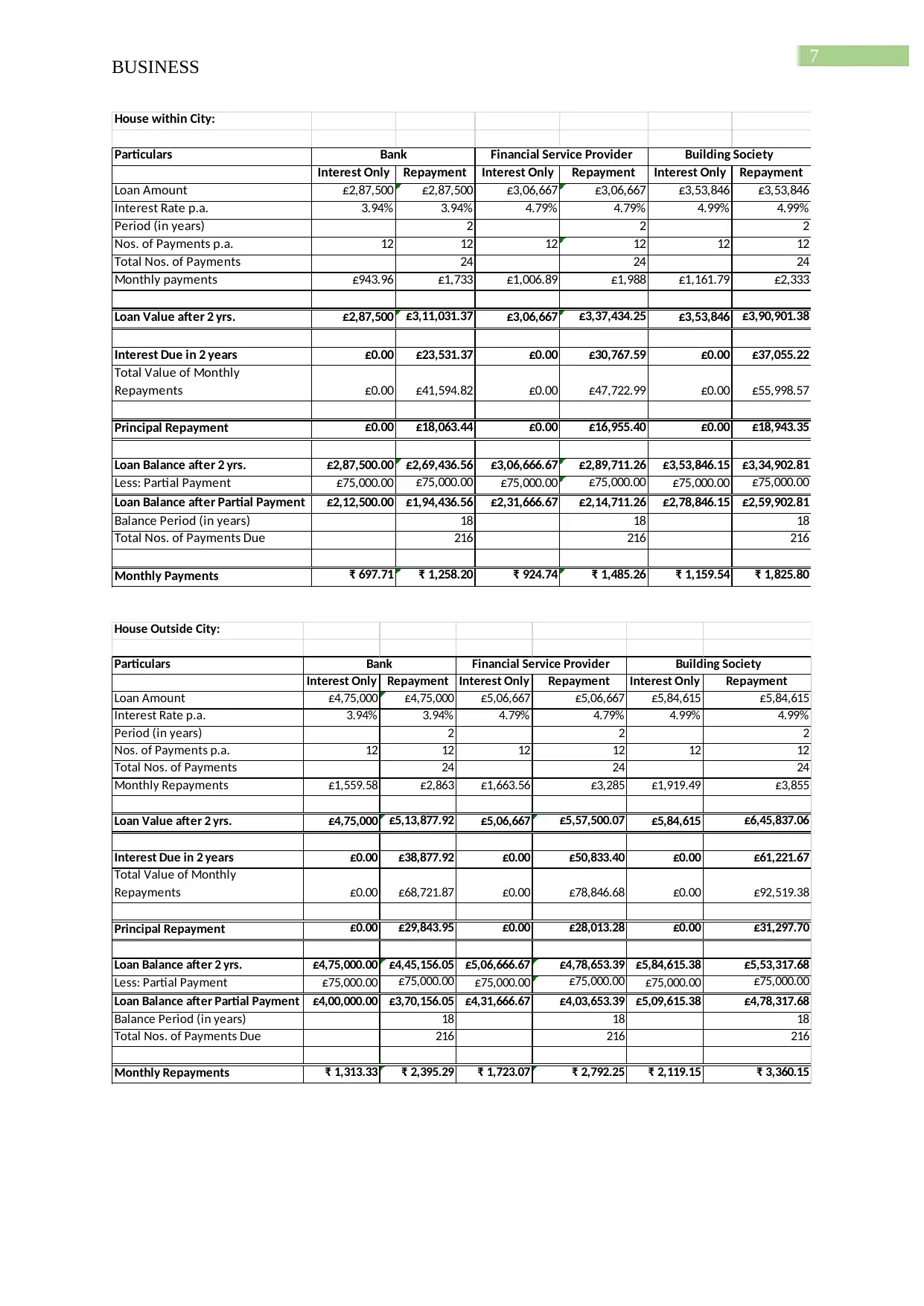
Requirement c)
Normal View:
Paraphrase This Document
Need a fresh take? Get an instant paraphrase of this document with our AI Paraphraser
7
BUSINESS
House within City:
Particulars
Interest Only Repayment Interest Only Repayment Interest Only Repayment
Loan Amount £2,87,500 £2,87,500 £3,06,667 £3,06,667 £3,53,846 £3,53,846
Interest Rate p.a. 3.94% 3.94% 4.79% 4.79% 4.99% 4.99%
Period (in years) 2 2 2
Nos. of Payments p.a. 12 12 12 12 12 12
Total Nos. of Payments 24 24 24
Monthly payments £943.96 £1,733 £1,006.89 £1,988 £1,161.79 £2,333
Loan Value after 2 yrs. £2,87,500 £3,11,031.37 £3,06,667 £3,37,434.25 £3,53,846 £3,90,901.38
Interest Due in 2 years £0.00 £23,531.37 £0.00 £30,767.59 £0.00 £37,055.22
Total Value of Monthly
Repayments £0.00 £41,594.82 £0.00 £47,722.99 £0.00 £55,998.57
Principal Repayment £0.00 £18,063.44 £0.00 £16,955.40 £0.00 £18,943.35
Loan Balance after 2 yrs. £2,87,500.00 £2,69,436.56 £3,06,666.67 £2,89,711.26 £3,53,846.15 £3,34,902.81
Less: Partial Payment £75,000.00 £75,000.00 £75,000.00 £75,000.00 £75,000.00 £75,000.00
Loan Balance after Partial Payment £2,12,500.00 £1,94,436.56 £2,31,666.67 £2,14,711.26 £2,78,846.15 £2,59,902.81
Balance Period (in years) 18 18 18
Total Nos. of Payments Due 216 216 216
Monthly Payments ₹ 697.71 ₹ 1,258.20 ₹ 924.74 ₹ 1,485.26 ₹ 1,159.54 ₹ 1,825.80
Bank Financial Service Provider Building Society
House Outside City:
Particulars
Interest Only Repayment Interest Only Repayment Interest Only Repayment
Loan Amount £4,75,000 £4,75,000 £5,06,667 £5,06,667 £5,84,615 £5,84,615
Interest Rate p.a. 3.94% 3.94% 4.79% 4.79% 4.99% 4.99%
Period (in years) 2 2 2
Nos. of Payments p.a. 12 12 12 12 12 12
Total Nos. of Payments 24 24 24
Monthly Repayments £1,559.58 £2,863 £1,663.56 £3,285 £1,919.49 £3,855
Loan Value after 2 yrs. £4,75,000 £5,13,877.92 £5,06,667 £5,57,500.07 £5,84,615 £6,45,837.06
Interest Due in 2 years £0.00 £38,877.92 £0.00 £50,833.40 £0.00 £61,221.67
Total Value of Monthly
Repayments £0.00 £68,721.87 £0.00 £78,846.68 £0.00 £92,519.38
Principal Repayment £0.00 £29,843.95 £0.00 £28,013.28 £0.00 £31,297.70
Loan Balance after 2 yrs. £4,75,000.00 £4,45,156.05 £5,06,666.67 £4,78,653.39 £5,84,615.38 £5,53,317.68
Less: Partial Payment £75,000.00 £75,000.00 £75,000.00 £75,000.00 £75,000.00 £75,000.00
Loan Balance after Partial Payment £4,00,000.00 £3,70,156.05 £4,31,666.67 £4,03,653.39 £5,09,615.38 £4,78,317.68
Balance Period (in years) 18 18 18
Total Nos. of Payments Due 216 216 216
Monthly Repayments ₹ 1,313.33 ₹ 2,395.29 ₹ 1,723.07 ₹ 2,792.25 ₹ 2,119.15 ₹ 3,360.15
Bank Financial Service Provider Building Society
8
BUSINESS
Formula View:
House within City:
Particulars
Interest Only Repayment Interest Only Repayment Interest Only Repayment
Loan Amount =C23 =C11 =E23 =E11 =G23 =G11
Interest Rate p.a. =C24 0.0394 =E24 0.0479 =G24 0.0499
Period (in years) 2 =C25 =E25
Nos. of Payments p.a. =C26 12 =E26 =C26 =G26 =E26
Total Nos. of Payments =C25*C26 =E25*E26 =G25*G26
Monthly payments =B17 =C17 =D17 =E17 =F17 =G17
Loan Value after 2 yrs. =B23 =FV((C24/12),C27,0,(-C23),0) =D23 =FV((E24/12),E27,0,(-E23),0) =F23 =FV((G24/12),G27,0,(-G23),0)
Interest Due in 2 years 0 =C30-C23 0 =E30-E23 0 =G30-G23
Total Value of Monthly Repayments 0 =C28*C27 0 =E28*E27 0 =G28*G27
Principal Repayment 0 =C33-C32 0 =E33-E32 0 =G33-G32
Loan Balance after 2 yrs. =B30-B35 =C23-C35 =D30-D35 =E23-E35 =F30-F35 =G23-G35
Less: Partial Payment =C38 75000 =E38 =C38 =G38 =E38
Loan Balance after Partial Payment =B37-B38 =C37-C38 =D37-D38 =E37-E38 =F37-F38 =G37-G38
Balance Period (in years) =20-C25 =20-E25 =20-G25
Total Nos. of Payments Due =C40*C26 =E40*E26 =G40*G26
Monthly Payments =B39*(B24/B26) =PMT((C24/C26),C41,(-C39),0)=D39*(D24/D26) =PMT((E24/E26),E41,(-E39),0) =F39*(F24/F26) =PMT((G24/G26),G41,(-G39),0)
Bank Financial Service Provider Building Society
House Outside City:
Particulars
Interest Only Repayment Interest Only Repayment Interest Only Repayment
Loan Amount =L23 =L11 =N23 =N11 =P23 =P11
Interest Rate p.a. =L24 0.0394 =N24 0.0479 =P24 0.0499
Period (in years) 2 =L25 =N25
Nos. of Payments p.a. =L26 12 =N26 =L26 =P26 =N26
Total Nos. of Payments =L25*L26 =N25*N26 =P25*P26
Monthly Repayments =K17 =L17 =M17 =N17 =O17 =P17
Loan Value after 2 yrs. =K23 =FV((L24/12),L27,0,(-L23),0) =M23 =FV((N24/12),N27,0,(-N23),0) =O23 =FV((P24/12),P27,0,(-P23),0)
Interest Due in 2 years 0 =L30-L23 0 =N30-N23 0 =P30-P23
Total Value of Monthly Repayments 0 =L28*L27 0 =N28*N27 0 =P28*P27
Principal Repayment 0 =L33-L32 0 =N33-N32 0 =P33-P32
Loan Balance after 2 yrs. =K30-K35 =L23-L35 =M30-M35 =N23-N35 =O30-O35 =P23-P35
Less: Partial Payment =L38 75000 =N38 =L38 =P38 =N38
Loan Balance after Partial Payment =K37-K38 =L37-L38 =M37-M38 =N37-N38 =O37-O38 =P37-P38
Balance Period (in years) =20-L25 =20-N25 =20-P25
Total Nos. of Payments Due =L40*L26 =N40*N26 =P40*P26
Monthly Repayments =K39*(K24/K26) =PMT((L24/L26),L41,(-L39),0)=M39*(M24/M26) =PMT((N24/N26),N41,(-N39),0) =O39*(O24/O26) =PMT((P24/P26),P41,(-P39),0)
Bank Financial Service Provider Building Society
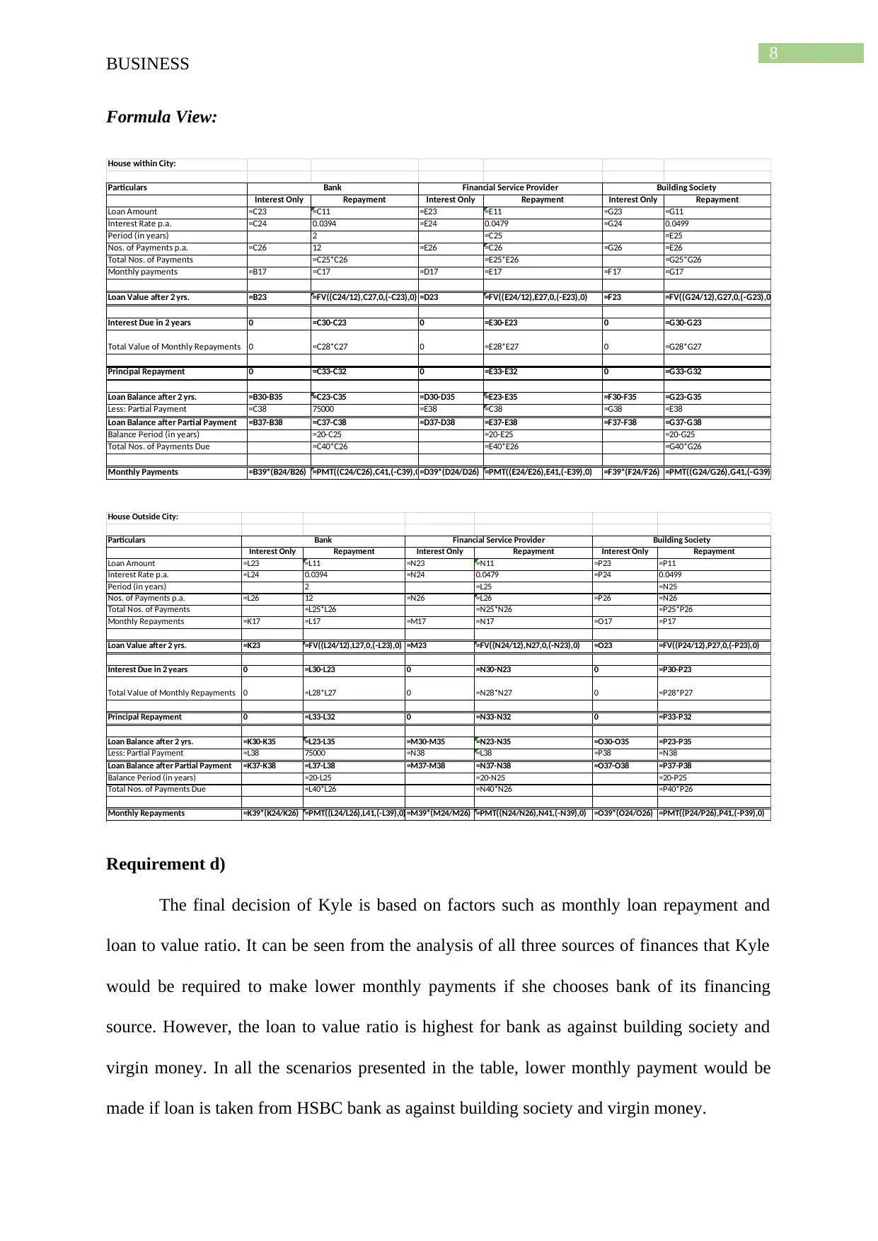
Requirement d)
The final decision of Kyle is based on factors such as monthly loan repayment and
loan to value ratio. It can be seen from the analysis of all three sources of finances that Kyle
would be required to make lower monthly payments if she chooses bank of its financing
source. However, the loan to value ratio is highest for bank as against building society and
virgin money. In all the scenarios presented in the table, lower monthly payment would be
made if loan is taken from HSBC bank as against building society and virgin money.
BUSINESS
Formula View:
House within City:
Particulars
Interest Only Repayment Interest Only Repayment Interest Only Repayment
Loan Amount =C23 =C11 =E23 =E11 =G23 =G11
Interest Rate p.a. =C24 0.0394 =E24 0.0479 =G24 0.0499
Period (in years) 2 =C25 =E25
Nos. of Payments p.a. =C26 12 =E26 =C26 =G26 =E26
Total Nos. of Payments =C25*C26 =E25*E26 =G25*G26
Monthly payments =B17 =C17 =D17 =E17 =F17 =G17
Loan Value after 2 yrs. =B23 =FV((C24/12),C27,0,(-C23),0) =D23 =FV((E24/12),E27,0,(-E23),0) =F23 =FV((G24/12),G27,0,(-G23),0)
Interest Due in 2 years 0 =C30-C23 0 =E30-E23 0 =G30-G23
Total Value of Monthly Repayments 0 =C28*C27 0 =E28*E27 0 =G28*G27
Principal Repayment 0 =C33-C32 0 =E33-E32 0 =G33-G32
Loan Balance after 2 yrs. =B30-B35 =C23-C35 =D30-D35 =E23-E35 =F30-F35 =G23-G35
Less: Partial Payment =C38 75000 =E38 =C38 =G38 =E38
Loan Balance after Partial Payment =B37-B38 =C37-C38 =D37-D38 =E37-E38 =F37-F38 =G37-G38
Balance Period (in years) =20-C25 =20-E25 =20-G25
Total Nos. of Payments Due =C40*C26 =E40*E26 =G40*G26
Monthly Payments =B39*(B24/B26) =PMT((C24/C26),C41,(-C39),0)=D39*(D24/D26) =PMT((E24/E26),E41,(-E39),0) =F39*(F24/F26) =PMT((G24/G26),G41,(-G39),0)
Bank Financial Service Provider Building Society
House Outside City:
Particulars
Interest Only Repayment Interest Only Repayment Interest Only Repayment
Loan Amount =L23 =L11 =N23 =N11 =P23 =P11
Interest Rate p.a. =L24 0.0394 =N24 0.0479 =P24 0.0499
Period (in years) 2 =L25 =N25
Nos. of Payments p.a. =L26 12 =N26 =L26 =P26 =N26
Total Nos. of Payments =L25*L26 =N25*N26 =P25*P26
Monthly Repayments =K17 =L17 =M17 =N17 =O17 =P17
Loan Value after 2 yrs. =K23 =FV((L24/12),L27,0,(-L23),0) =M23 =FV((N24/12),N27,0,(-N23),0) =O23 =FV((P24/12),P27,0,(-P23),0)
Interest Due in 2 years 0 =L30-L23 0 =N30-N23 0 =P30-P23
Total Value of Monthly Repayments 0 =L28*L27 0 =N28*N27 0 =P28*P27
Principal Repayment 0 =L33-L32 0 =N33-N32 0 =P33-P32
Loan Balance after 2 yrs. =K30-K35 =L23-L35 =M30-M35 =N23-N35 =O30-O35 =P23-P35
Less: Partial Payment =L38 75000 =N38 =L38 =P38 =N38
Loan Balance after Partial Payment =K37-K38 =L37-L38 =M37-M38 =N37-N38 =O37-O38 =P37-P38
Balance Period (in years) =20-L25 =20-N25 =20-P25
Total Nos. of Payments Due =L40*L26 =N40*N26 =P40*P26
Monthly Repayments =K39*(K24/K26) =PMT((L24/L26),L41,(-L39),0)=M39*(M24/M26) =PMT((N24/N26),N41,(-N39),0) =O39*(O24/O26) =PMT((P24/P26),P41,(-P39),0)
Bank Financial Service Provider Building Society
Requirement d)
The final decision of Kyle is based on factors such as monthly loan repayment and
loan to value ratio. It can be seen from the analysis of all three sources of finances that Kyle
would be required to make lower monthly payments if she chooses bank of its financing
source. However, the loan to value ratio is highest for bank as against building society and
virgin money. In all the scenarios presented in the table, lower monthly payment would be
made if loan is taken from HSBC bank as against building society and virgin money.
⊘ This is a preview!⊘
Do you want full access?
Subscribe today to unlock all pages.
Trusted by 1+ million students worldwide
9
BUSINESS
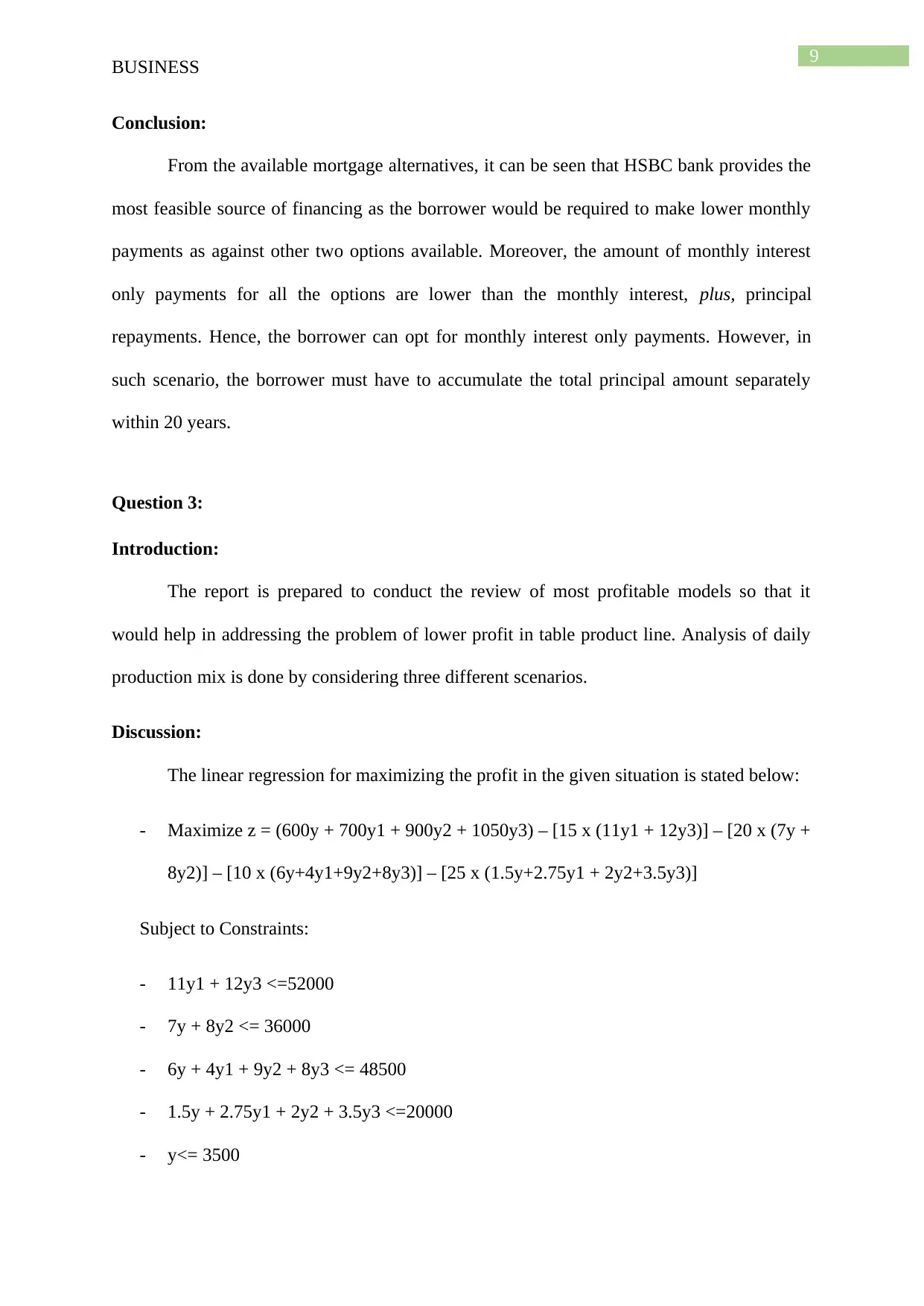
Conclusion:
From the available mortgage alternatives, it can be seen that HSBC bank provides the
most feasible source of financing as the borrower would be required to make lower monthly
payments as against other two options available. Moreover, the amount of monthly interest
only payments for all the options are lower than the monthly interest, plus, principal
repayments. Hence, the borrower can opt for monthly interest only payments. However, in
such scenario, the borrower must have to accumulate the total principal amount separately
within 20 years.
Question 3:
Introduction:
The report is prepared to conduct the review of most profitable models so that it
would help in addressing the problem of lower profit in table product line. Analysis of daily
production mix is done by considering three different scenarios.
Discussion:
The linear regression for maximizing the profit in the given situation is stated below:
- Maximize z = (600y + 700y1 + 900y2 + 1050y3) – [15 x (11y1 + 12y3)] – [20 x (7y +
8y2)] – [10 x (6y+4y1+9y2+8y3)] – [25 x (1.5y+2.75y1 + 2y2+3.5y3)]
Subject to Constraints:
- 11y1 + 12y3 <=52000
- 7y + 8y2 <= 36000
- 6y + 4y1 + 9y2 + 8y3 <= 48500
- 1.5y + 2.75y1 + 2y2 + 3.5y3 <=20000
- y<= 3500
BUSINESS
Conclusion:
From the available mortgage alternatives, it can be seen that HSBC bank provides the
most feasible source of financing as the borrower would be required to make lower monthly
payments as against other two options available. Moreover, the amount of monthly interest
only payments for all the options are lower than the monthly interest, plus, principal
repayments. Hence, the borrower can opt for monthly interest only payments. However, in
such scenario, the borrower must have to accumulate the total principal amount separately
within 20 years.
Question 3:
Introduction:
The report is prepared to conduct the review of most profitable models so that it
would help in addressing the problem of lower profit in table product line. Analysis of daily
production mix is done by considering three different scenarios.
Discussion:
The linear regression for maximizing the profit in the given situation is stated below:
- Maximize z = (600y + 700y1 + 900y2 + 1050y3) – [15 x (11y1 + 12y3)] – [20 x (7y +
8y2)] – [10 x (6y+4y1+9y2+8y3)] – [25 x (1.5y+2.75y1 + 2y2+3.5y3)]
Subject to Constraints:
- 11y1 + 12y3 <=52000
- 7y + 8y2 <= 36000
- 6y + 4y1 + 9y2 + 8y3 <= 48500
- 1.5y + 2.75y1 + 2y2 + 3.5y3 <=20000
- y<= 3500
Paraphrase This Document
Need a fresh take? Get an instant paraphrase of this document with our AI Paraphraser
10
BUSINESS
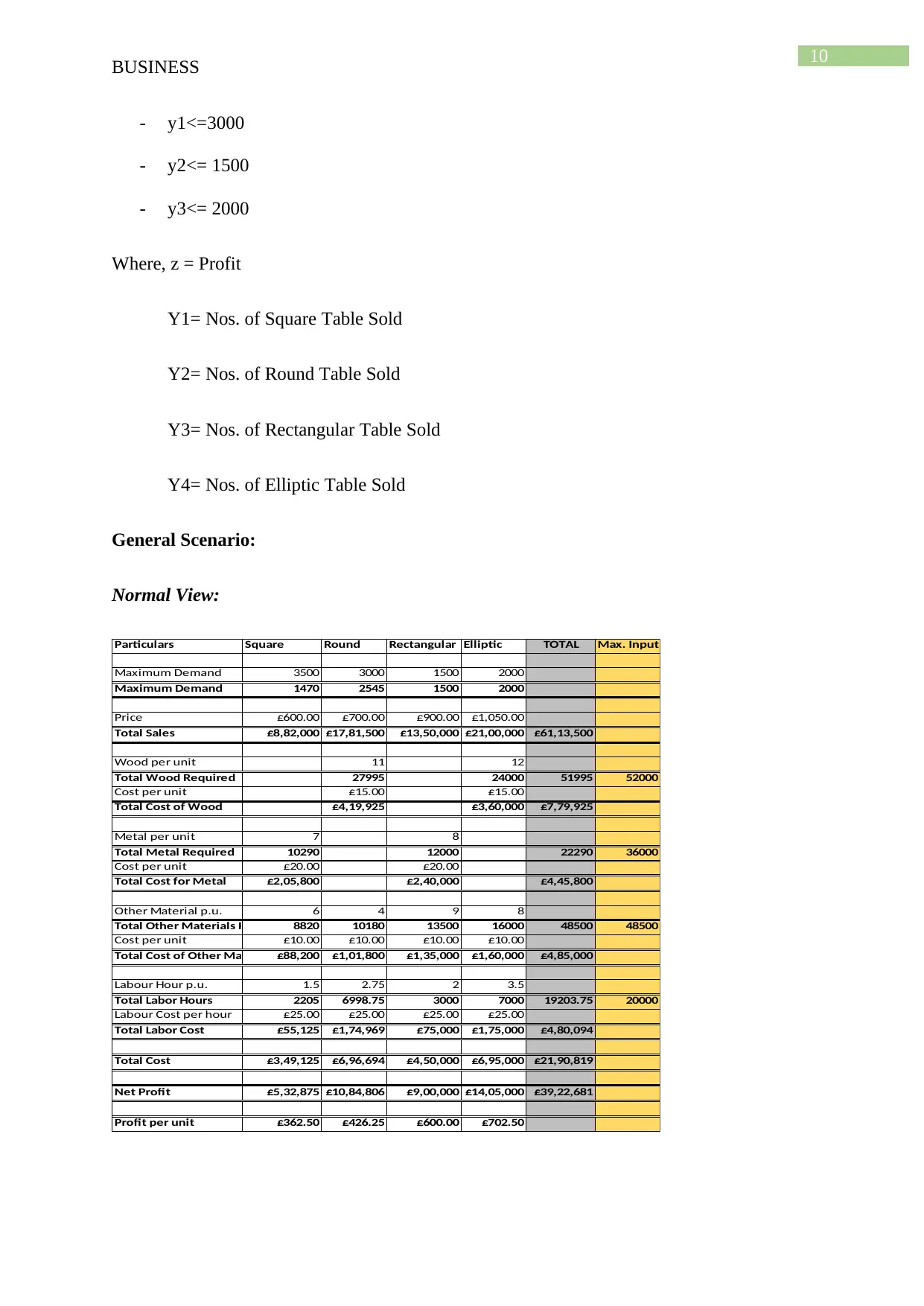
- y1<=3000
- y2<= 1500
- y3<= 2000
Where, z = Profit
Y1= Nos. of Square Table Sold
Y2= Nos. of Round Table Sold
Y3= Nos. of Rectangular Table Sold
Y4= Nos. of Elliptic Table Sold
General Scenario:
Normal View:
Particulars Square Round Rectangular Elliptic TOTAL Max. Input
Maximum Demand 3500 3000 1500 2000
Maximum Demand 1470 2545 1500 2000
Price £600.00 £700.00 £900.00 £1,050.00
Total Sales £8,82,000 £17,81,500 £13,50,000 £21,00,000 £61,13,500
Wood per unit 11 12
Total Wood Required 27995 24000 51995 52000
Cost per unit £15.00 £15.00
Total Cost of Wood £4,19,925 £3,60,000 £7,79,925
Metal per unit 7 8
Total Metal Required 10290 12000 22290 36000
Cost per unit £20.00 £20.00
Total Cost for Metal £2,05,800 £2,40,000 £4,45,800
Other Material p.u. 6 4 9 8
Total Other Materials Required 8820 10180 13500 16000 48500 48500
Cost per unit £10.00 £10.00 £10.00 £10.00
Total Cost of Other Material £88,200 £1,01,800 £1,35,000 £1,60,000 £4,85,000
Labour Hour p.u. 1.5 2.75 2 3.5
Total Labor Hours 2205 6998.75 3000 7000 19203.75 20000
Labour Cost per hour £25.00 £25.00 £25.00 £25.00
Total Labor Cost £55,125 £1,74,969 £75,000 £1,75,000 £4,80,094
Total Cost £3,49,125 £6,96,694 £4,50,000 £6,95,000 £21,90,819
Net Profit £5,32,875 £10,84,806 £9,00,000 £14,05,000 £39,22,681
Profit per unit £362.50 £426.25 £600.00 £702.50
BUSINESS
- y1<=3000
- y2<= 1500
- y3<= 2000
Where, z = Profit
Y1= Nos. of Square Table Sold
Y2= Nos. of Round Table Sold
Y3= Nos. of Rectangular Table Sold
Y4= Nos. of Elliptic Table Sold
General Scenario:
Normal View:
Particulars Square Round Rectangular Elliptic TOTAL Max. Input
Maximum Demand 3500 3000 1500 2000
Maximum Demand 1470 2545 1500 2000
Price £600.00 £700.00 £900.00 £1,050.00
Total Sales £8,82,000 £17,81,500 £13,50,000 £21,00,000 £61,13,500
Wood per unit 11 12
Total Wood Required 27995 24000 51995 52000
Cost per unit £15.00 £15.00
Total Cost of Wood £4,19,925 £3,60,000 £7,79,925
Metal per unit 7 8
Total Metal Required 10290 12000 22290 36000
Cost per unit £20.00 £20.00
Total Cost for Metal £2,05,800 £2,40,000 £4,45,800
Other Material p.u. 6 4 9 8
Total Other Materials Required 8820 10180 13500 16000 48500 48500
Cost per unit £10.00 £10.00 £10.00 £10.00
Total Cost of Other Material £88,200 £1,01,800 £1,35,000 £1,60,000 £4,85,000
Labour Hour p.u. 1.5 2.75 2 3.5
Total Labor Hours 2205 6998.75 3000 7000 19203.75 20000
Labour Cost per hour £25.00 £25.00 £25.00 £25.00
Total Labor Cost £55,125 £1,74,969 £75,000 £1,75,000 £4,80,094
Total Cost £3,49,125 £6,96,694 £4,50,000 £6,95,000 £21,90,819
Net Profit £5,32,875 £10,84,806 £9,00,000 £14,05,000 £39,22,681
Profit per unit £362.50 £426.25 £600.00 £702.50
11
BUSINESS
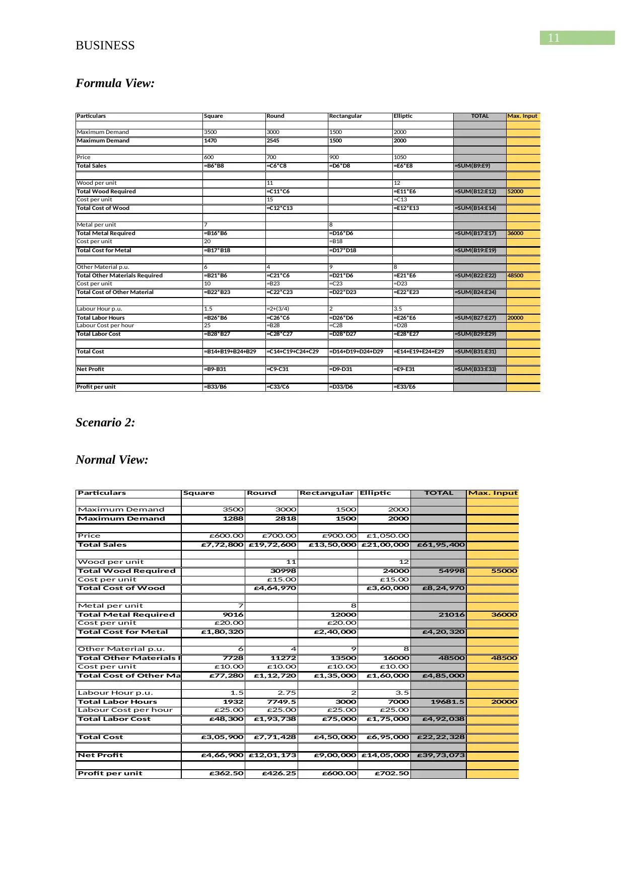
Formula View:
Particulars Square Round Rectangular Elliptic TOTAL Max. Input
Maximum Demand 3500 3000 1500 2000
Maximum Demand 1470 2545 1500 2000
Price 600 700 900 1050
Total Sales =B6*B8 =C6*C8 =D6*D8 =E6*E8 =SUM(B9:E9)
Wood per unit 11 12
Total Wood Required =C11*C6 =E11*E6 =SUM(B12:E12) 52000
Cost per unit 15 =C13
Total Cost of Wood =C12*C13 =E12*E13 =SUM(B14:E14)
Metal per unit 7 8
Total Metal Required =B16*B6 =D16*D6 =SUM(B17:E17) 36000
Cost per unit 20 =B18
Total Cost for Metal =B17*B18 =D17*D18 =SUM(B19:E19)
Other Material p.u. 6 4 9 8
Total Other Materials Required =B21*B6 =C21*C6 =D21*D6 =E21*E6 =SUM(B22:E22) 48500
Cost per unit 10 =B23 =C23 =D23
Total Cost of Other Material =B22*B23 =C22*C23 =D22*D23 =E22*E23 =SUM(B24:E24)
Labour Hour p.u. 1.5 =2+(3/4) 2 3.5
Total Labor Hours =B26*B6 =C26*C6 =D26*D6 =E26*E6 =SUM(B27:E27) 20000
Labour Cost per hour 25 =B28 =C28 =D28
Total Labor Cost =B28*B27 =C28*C27 =D28*D27 =E28*E27 =SUM(B29:E29)
Total Cost =B14+B19+B24+B29 =C14+C19+C24+C29 =D14+D19+D24+D29 =E14+E19+E24+E29 =SUM(B31:E31)
Net Profit =B9-B31 =C9-C31 =D9-D31 =E9-E31 =SUM(B33:E33)
Profit per unit =B33/B6 =C33/C6 =D33/D6 =E33/E6
Scenario 2:
Normal View:
Particulars Square Round Rectangular Elliptic TOTAL Max. Input
Maximum Demand 3500 3000 1500 2000
Maximum Demand 1288 2818 1500 2000
Price £600.00 £700.00 £900.00 £1,050.00
Total Sales £7,72,800 £19,72,600 £13,50,000 £21,00,000 £61,95,400
Wood per unit 11 12
Total Wood Required 30998 24000 54998 55000
Cost per unit £15.00 £15.00
Total Cost of Wood £4,64,970 £3,60,000 £8,24,970
Metal per unit 7 8
Total Metal Required 9016 12000 21016 36000
Cost per unit £20.00 £20.00
Total Cost for Metal £1,80,320 £2,40,000 £4,20,320
Other Material p.u. 6 4 9 8
Total Other Materials Required 7728 11272 13500 16000 48500 48500
Cost per unit £10.00 £10.00 £10.00 £10.00
Total Cost of Other Material £77,280 £1,12,720 £1,35,000 £1,60,000 £4,85,000
Labour Hour p.u. 1.5 2.75 2 3.5
Total Labor Hours 1932 7749.5 3000 7000 19681.5 20000
Labour Cost per hour £25.00 £25.00 £25.00 £25.00
Total Labor Cost £48,300 £1,93,738 £75,000 £1,75,000 £4,92,038
Total Cost £3,05,900 £7,71,428 £4,50,000 £6,95,000 £22,22,328
Net Profit £4,66,900 £12,01,173 £9,00,000 £14,05,000 £39,73,073
Profit per unit £362.50 £426.25 £600.00 £702.50
BUSINESS
Formula View:
Particulars Square Round Rectangular Elliptic TOTAL Max. Input
Maximum Demand 3500 3000 1500 2000
Maximum Demand 1470 2545 1500 2000
Price 600 700 900 1050
Total Sales =B6*B8 =C6*C8 =D6*D8 =E6*E8 =SUM(B9:E9)
Wood per unit 11 12
Total Wood Required =C11*C6 =E11*E6 =SUM(B12:E12) 52000
Cost per unit 15 =C13
Total Cost of Wood =C12*C13 =E12*E13 =SUM(B14:E14)
Metal per unit 7 8
Total Metal Required =B16*B6 =D16*D6 =SUM(B17:E17) 36000
Cost per unit 20 =B18
Total Cost for Metal =B17*B18 =D17*D18 =SUM(B19:E19)
Other Material p.u. 6 4 9 8
Total Other Materials Required =B21*B6 =C21*C6 =D21*D6 =E21*E6 =SUM(B22:E22) 48500
Cost per unit 10 =B23 =C23 =D23
Total Cost of Other Material =B22*B23 =C22*C23 =D22*D23 =E22*E23 =SUM(B24:E24)
Labour Hour p.u. 1.5 =2+(3/4) 2 3.5
Total Labor Hours =B26*B6 =C26*C6 =D26*D6 =E26*E6 =SUM(B27:E27) 20000
Labour Cost per hour 25 =B28 =C28 =D28
Total Labor Cost =B28*B27 =C28*C27 =D28*D27 =E28*E27 =SUM(B29:E29)
Total Cost =B14+B19+B24+B29 =C14+C19+C24+C29 =D14+D19+D24+D29 =E14+E19+E24+E29 =SUM(B31:E31)
Net Profit =B9-B31 =C9-C31 =D9-D31 =E9-E31 =SUM(B33:E33)
Profit per unit =B33/B6 =C33/C6 =D33/D6 =E33/E6
Scenario 2:
Normal View:
Particulars Square Round Rectangular Elliptic TOTAL Max. Input
Maximum Demand 3500 3000 1500 2000
Maximum Demand 1288 2818 1500 2000
Price £600.00 £700.00 £900.00 £1,050.00
Total Sales £7,72,800 £19,72,600 £13,50,000 £21,00,000 £61,95,400
Wood per unit 11 12
Total Wood Required 30998 24000 54998 55000
Cost per unit £15.00 £15.00
Total Cost of Wood £4,64,970 £3,60,000 £8,24,970
Metal per unit 7 8
Total Metal Required 9016 12000 21016 36000
Cost per unit £20.00 £20.00
Total Cost for Metal £1,80,320 £2,40,000 £4,20,320
Other Material p.u. 6 4 9 8
Total Other Materials Required 7728 11272 13500 16000 48500 48500
Cost per unit £10.00 £10.00 £10.00 £10.00
Total Cost of Other Material £77,280 £1,12,720 £1,35,000 £1,60,000 £4,85,000
Labour Hour p.u. 1.5 2.75 2 3.5
Total Labor Hours 1932 7749.5 3000 7000 19681.5 20000
Labour Cost per hour £25.00 £25.00 £25.00 £25.00
Total Labor Cost £48,300 £1,93,738 £75,000 £1,75,000 £4,92,038
Total Cost £3,05,900 £7,71,428 £4,50,000 £6,95,000 £22,22,328
Net Profit £4,66,900 £12,01,173 £9,00,000 £14,05,000 £39,73,073
Profit per unit £362.50 £426.25 £600.00 £702.50
⊘ This is a preview!⊘
Do you want full access?
Subscribe today to unlock all pages.
Trusted by 1+ million students worldwide
1 out of 23

Your All-in-One AI-Powered Toolkit for Academic Success.
+13062052269
info@desklib.com
Available 24*7 on WhatsApp / Email
![[object Object]](/_next/static/media/star-bottom.7253800d.svg)
Unlock your academic potential
Copyright © 2020–2026 A2Z Services. All Rights Reserved. Developed and managed by ZUCOL.