Control System Design and Simulation for Inverted Pendulum Project
VerifiedAdded on 2023/04/21
|31
|3267
|118
Project
AI Summary
This project report details the design and analysis of a control system for a rotary inverted pendulum. It begins with an introduction to the problem and aims to design a controller using a linearized pendulum model. The report outlines the steps to build a Simulink model of the inverted pendulum, including the use of Fcn blocks, Integrator blocks, Multiplexer blocks, and various equations. The report then analyzes the system's response to impulse disturbances and step commands, defining performance requirements such as settling time and pendulum angle limitations. It covers linearization techniques and the use of state-space methods for controller design, including pole placement. MATLAB commands and the Control System Designer are used to implement and analyze the controller. The project explores open-loop and closed-loop responses, including impulse responses, pole-zero maps, Bode plots, and Nyquist diagrams. Discrete-time system responses and Simulink simulations are also provided to compare real-time and simulated results. The report concludes with a summary of the findings and references relevant research papers.

University
*** Semester
Inverted Pendulum
Student Name:
Register Number:
Submission Date:
*** Semester
Inverted Pendulum
Student Name:
Register Number:
Submission Date:
Paraphrase This Document
Need a fresh take? Get an instant paraphrase of this document with our AI Paraphraser

Table of Contents
Question-1.................................................................................................................................................................... 1
Question-2.................................................................................................................................................................... 1
Question-3.................................................................................................................................................................... 2
Question-4.................................................................................................................................................................... 3
Question-5.................................................................................................................................................................... 5
Question-6.................................................................................................................................................................... 6
Question-7.................................................................................................................................................................... 8
Question-8.................................................................................................................................................................. 10
Question-9.................................................................................................................................................................. 12
Output Graphs............................................................................................................................................................... 14
Step Input to the System............................................................................................................................................ 14
Response of pendulum position to an Impulse Disturbance.........................................................................................15
Pole – zero map of the System..................................................................................................................................... 15
Step Response with estimator...................................................................................................................................... 16
Real Pole plot.............................................................................................................................................................. 16
Complex pole plot....................................................................................................................................................... 17
Real zero plot.............................................................................................................................................................. 17
Complex zero plot....................................................................................................................................................... 18
Integrator plot............................................................................................................................................................ 18
Differentiator Plot....................................................................................................................................................... 19
Notch filter with zero and pole plot............................................................................................................................. 19
Open loop of Bode plot............................................................................................................................................... 20
Open Loop of Nyquist Diagram.................................................................................................................................. 20
Closed Loop response of Bode and Nyquist plot..........................................................................................................21
Discrete -time system response of Inverted Pendulum.................................................................................................21
Input – Output Plot of Pendulum position...................................................................................................................22
Simulation of Simulink Model of the Inverted Pendulum............................................................................................22
Step response comparison........................................................................................................................................... 23
Change in position of pendulum at a point..................................................................................................................23
Impulse disturbance rejection in a pendulum..............................................................................................................24
Summary....................................................................................................................................................................... 24
References...................................................................................................................................................................... 25

⊘ This is a preview!⊘
Do you want full access?
Subscribe today to unlock all pages.
Trusted by 1+ million students worldwide

Question-1
ANSWER:
Introduction
The Rotary Inverted Pendulum is an exemplary control issue that is investigated
frequently as an undertaking in control courses because of its effectively created elements that
area mix of its multifaceted nature of control design 1. It is a system which is built using the
pendulum that is attached to the rotary arm’s end, which the motor controls. In general, the motor
includes the servomotor coupled, by using the gear-chain. The principle objective includes
keeping the pendulum in the upright position of unsteady equilibrium. The next objective
includes keeping the motor at the specifically mentioned angular position, when the first task is
being performed. Whereas, the last task includes destabilizing the motor starting from the
hanging position of the equilibrium which is not stable, with the goal to achieve the stability
range (i.e., here the mode controller could easily start the stabilization.) 2.
Aim
The aimincludesdesigning the controller for the ROTPEN kit, with the help of an
effective linearised pendulum model.
Question-2
ANSWER:
The below mentioned steps help to build the inverted pendulum model in Simulink, they
are 3,
1 P S A, "THE STABILIZATION OF FORCED INVERTED PENDULUM VIA FUZZY CONTROLLER",
in International Journal of Research in Engineering and Technology, vol. 05, 2016, 152-155.
2 J Babu & E Vargheese, "Stabilization of Rotary Arm Inverted Pendulum using State Feedback
Techniques", in International Journal of Engineering Research and, vol. V4, 2015.
3 H Ali, "Robust Stabilizing Controller Design for Inverted Pendulum System", in Jurnal Teknologi, vol. 71,
2014.
1
ANSWER:
Introduction
The Rotary Inverted Pendulum is an exemplary control issue that is investigated
frequently as an undertaking in control courses because of its effectively created elements that
area mix of its multifaceted nature of control design 1. It is a system which is built using the
pendulum that is attached to the rotary arm’s end, which the motor controls. In general, the motor
includes the servomotor coupled, by using the gear-chain. The principle objective includes
keeping the pendulum in the upright position of unsteady equilibrium. The next objective
includes keeping the motor at the specifically mentioned angular position, when the first task is
being performed. Whereas, the last task includes destabilizing the motor starting from the
hanging position of the equilibrium which is not stable, with the goal to achieve the stability
range (i.e., here the mode controller could easily start the stabilization.) 2.
Aim
The aimincludesdesigning the controller for the ROTPEN kit, with the help of an
effective linearised pendulum model.
Question-2
ANSWER:
The below mentioned steps help to build the inverted pendulum model in Simulink, they
are 3,
1 P S A, "THE STABILIZATION OF FORCED INVERTED PENDULUM VIA FUZZY CONTROLLER",
in International Journal of Research in Engineering and Technology, vol. 05, 2016, 152-155.
2 J Babu & E Vargheese, "Stabilization of Rotary Arm Inverted Pendulum using State Feedback
Techniques", in International Journal of Engineering Research and, vol. V4, 2015.
3 H Ali, "Robust Stabilizing Controller Design for Inverted Pendulum System", in Jurnal Teknologi, vol. 71,
2014.
1
Paraphrase This Document
Need a fresh take? Get an instant paraphrase of this document with our AI Paraphraser

1) In the MATLAB command window type Simulink and it opens the Simulink
environment. Next,in Simulink open a new model window by selecting New >
Simulink > Blank Model of the open Simulink Start Page window or by
pressing Ctrl-N.
2) From the Simulink/User-Defined Functions library, 4 Fcn Blocks are inserted. The
following equations for , , , and are built by employing the blocks.
3) Every single Fcn block must be changed so that itmatches with its linked function.
4) From the Simulink/Continuous library4 Integrator blocks must be inserted. Every
single Integrator block’s output will be the system’s state variable, , , , and .
5) Every single Integrator block must be double-clicked for adding the “State Name:” of
the linked state variable. Next, the “Initial condition:”must be changedfor
(pendulum angle) to "pi", for representing that the pendulum starts to point straight up.
6) From the Simulink/Signal Routing library, 4 Multiplexer (Mux) blocks must be
inserted, for every single Fcn block.
7) From the Simulink/Sinks and Simulink/Sources libraries, 2 Out1 blocks and one In1
block must be inserted, respectively. Next, the labels must be double-clicked, as it
helps to change the names of the blocks. For "Position" of the cart and the "Angle" of
the pendulum, two outputs are provided when one input is for "Force" that is applied
on the cart.
8) Mux blocks’ each output is connected to the corresponding input of the Fcn block.
9) In the function blocks the below equations are filled 4.
( J eq+ M p r2 ) ¨θ + M p Lp rsinα ( ˙α )2−M p Lp rcosα ¨α=τ output−β1 ˙θ
4
3 M p Lp
2 ¨α −M p Lp rcosα ¨θ−Mp g Lp sinα=− β2 ˙α
τ output= Kt [ V m−Km ˙θ (t) ]
Rm
4 L Wan, J Lei & H Wu, "Design of LQR Controller for the Inverted Pendulum", in Advanced Materials
Research, vol. 1037, 2014, 221-224.
2
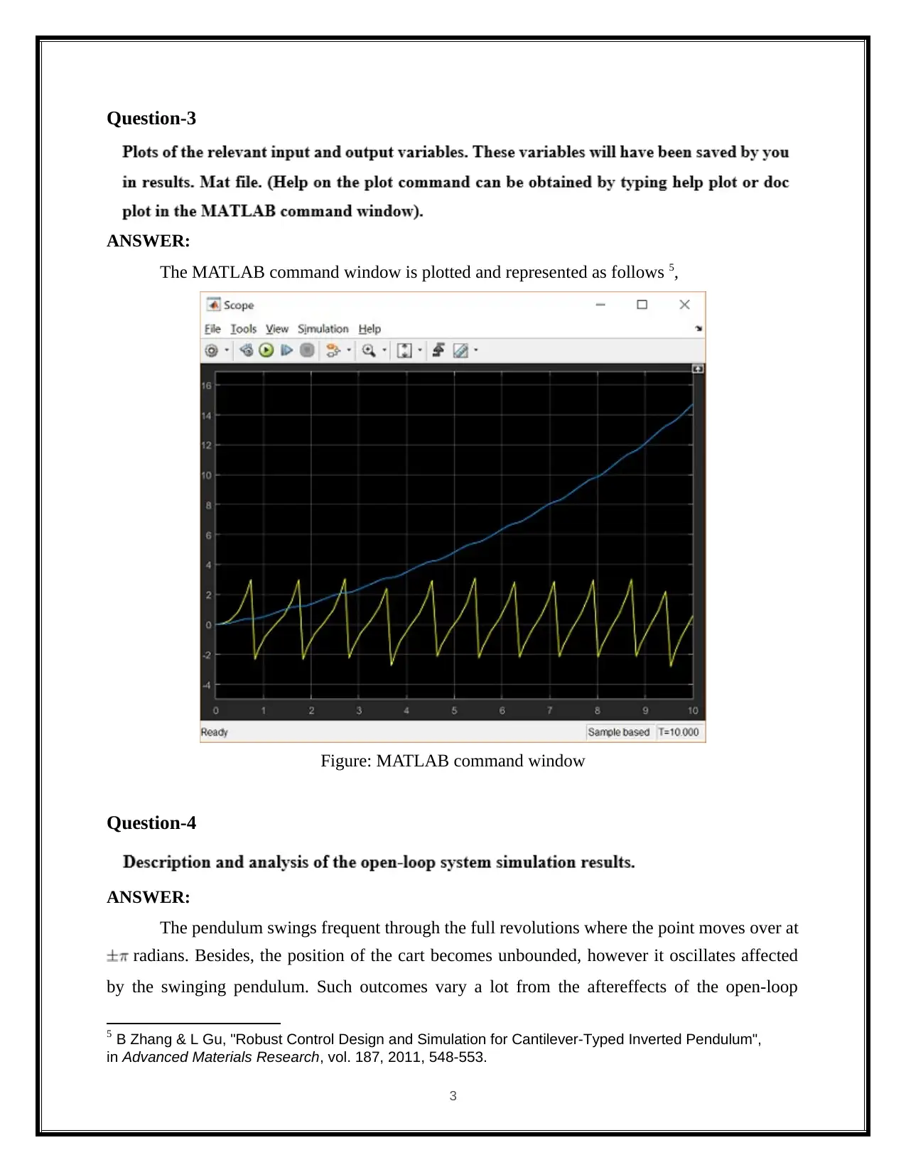
Question-3
ANSWER:
The MATLAB command window is plotted and represented as follows 5,
Figure: MATLAB command window
Question-4
ANSWER:
The pendulum swings frequent through the full revolutions where the point moves over at
radians. Besides, the position of the cart becomes unbounded, however it oscillates affected
by the swinging pendulum. Such outcomes vary a lot from the aftereffects of the open-loop
5 B Zhang & L Gu, "Robust Control Design and Simulation for Cantilever-Typed Inverted Pendulum",
in Advanced Materials Research, vol. 187, 2011, 548-553.
3
ANSWER:
The MATLAB command window is plotted and represented as follows 5,
Figure: MATLAB command window
Question-4
ANSWER:
The pendulum swings frequent through the full revolutions where the point moves over at
radians. Besides, the position of the cart becomes unbounded, however it oscillates affected
by the swinging pendulum. Such outcomes vary a lot from the aftereffects of the open-loop
5 B Zhang & L Gu, "Robust Control Design and Simulation for Cantilever-Typed Inverted Pendulum",
in Advanced Materials Research, vol. 187, 2011, 548-553.
3
⊘ This is a preview!⊘
Do you want full access?
Subscribe today to unlock all pages.
Trusted by 1+ million students worldwide
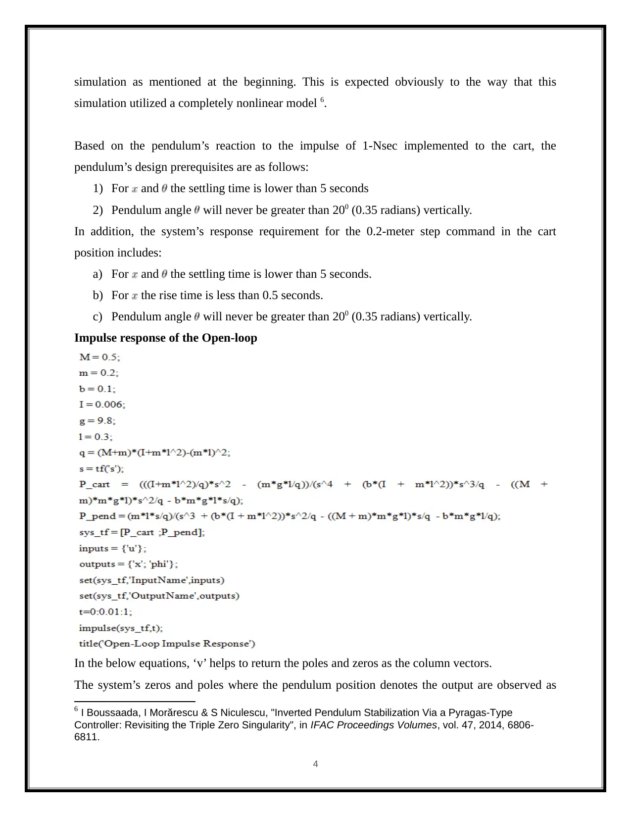
simulation as mentioned at the beginning. This is expected obviously to the way that this
simulation utilized a completely nonlinear model 6.
Based on the pendulum’s reaction to the impulse of 1-Nsec implemented to the cart, the
pendulum’s design prerequisites are as follows:
1) For and the settling time is lower than 5 seconds
2) Pendulum angle will never be greater than 200 (0.35 radians) vertically.
In addition, the system’s response requirement for the 0.2-meter step command in the cart
position includes:
a) For and the settling time is lower than 5 seconds.
b) For the rise time is less than 0.5 seconds.
c) Pendulum angle will never be greater than 200 (0.35 radians) vertically.
Impulse response of the Open-loop
In the below equations, ‘v’ helps to return the poles and zeros as the column vectors.
The system’s zeros and poles where the pendulum position denotes the output are observed as
6 I Boussaada, I Morărescu & S Niculescu, "Inverted Pendulum Stabilization Via a Pyragas-Type
Controller: Revisiting the Triple Zero Singularity", in IFAC Proceedings Volumes, vol. 47, 2014, 6806-
6811.
4
Paraphrase This Document
Need a fresh take? Get an instant paraphrase of this document with our AI Paraphraser
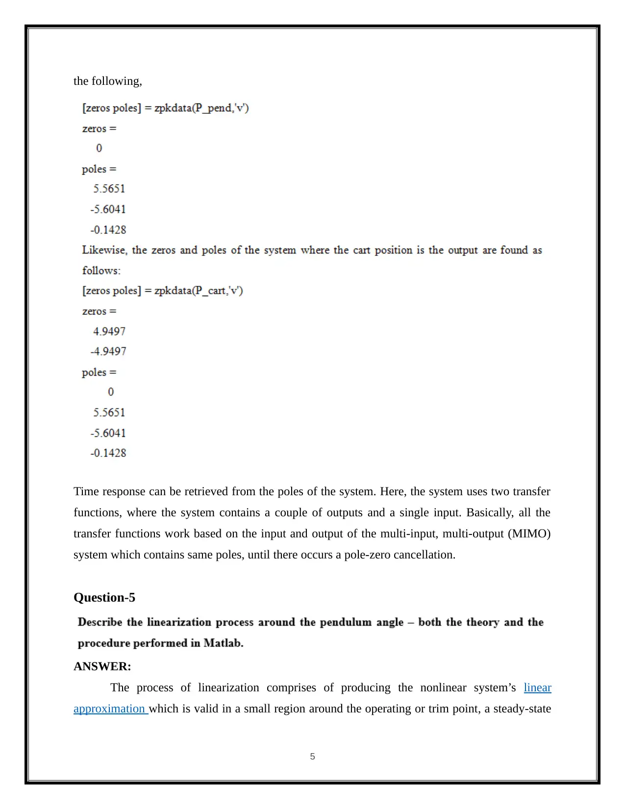
the following,
Time response can be retrieved from the poles of the system. Here, the system uses two transfer
functions, where the system contains a couple of outputs and a single input. Basically, all the
transfer functions work based on the input and output of the multi-input, multi-output (MIMO)
system which contains same poles, until there occurs a pole-zero cancellation.
Question-5
ANSWER:
The process of linearization comprises of producing the nonlinear system’s linear
approximation which is valid in a small region around the operating or trim point, a steady-state
5
condition, where all the model states are constant(Wang & Hu, 2014).For designing the control
system linearization is required, which uses the classical design methods like root locus design
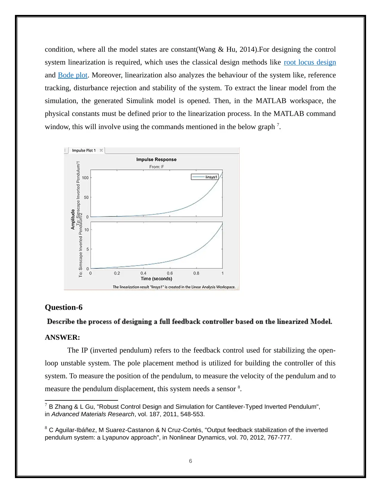
and Bode plot. Moreover, linearization also analyzes the behaviour of the system like, reference
tracking, disturbance rejection and stability of the system. To extract the linear model from the
simulation, the generated Simulink model is opened. Then, in the MATLAB workspace, the
physical constants must be defined prior to the linearization process. In the MATLAB command
window, this will involve using the commands mentioned in the below graph 7.
Question-6
ANSWER:
The IP (inverted pendulum) refers to the feedback control used for stabilizing the open-
loop unstable system. The pole placement method is utilized for building the controller of this
system. To measure the position of the pendulum, to measure the velocity of the pendulum and to
measure the pendulum displacement, this system needs a sensor 8.
7 B Zhang & L Gu, "Robust Control Design and Simulation for Cantilever-Typed Inverted Pendulum",
in Advanced Materials Research, vol. 187, 2011, 548-553.
8 C Aguilar-Ibáñez, M Suarez-Castanon & N Cruz-Cortés, "Output feedback stabilization of the inverted
pendulum system: a Lyapunov approach", in Nonlinear Dynamics, vol. 70, 2012, 767-777.
6
system linearization is required, which uses the classical design methods like root locus design
and Bode plot. Moreover, linearization also analyzes the behaviour of the system like, reference
tracking, disturbance rejection and stability of the system. To extract the linear model from the
simulation, the generated Simulink model is opened. Then, in the MATLAB workspace, the
physical constants must be defined prior to the linearization process. In the MATLAB command
window, this will involve using the commands mentioned in the below graph 7.
Question-6
ANSWER:
The IP (inverted pendulum) refers to the feedback control used for stabilizing the open-
loop unstable system. The pole placement method is utilized for building the controller of this
system. To measure the position of the pendulum, to measure the velocity of the pendulum and to
measure the pendulum displacement, this system needs a sensor 8.
7 B Zhang & L Gu, "Robust Control Design and Simulation for Cantilever-Typed Inverted Pendulum",
in Advanced Materials Research, vol. 187, 2011, 548-553.
8 C Aguilar-Ibáñez, M Suarez-Castanon & N Cruz-Cortés, "Output feedback stabilization of the inverted
pendulum system: a Lyapunov approach", in Nonlinear Dynamics, vol. 70, 2012, 767-777.
6
⊘ This is a preview!⊘
Do you want full access?
Subscribe today to unlock all pages.
Trusted by 1+ million students worldwide
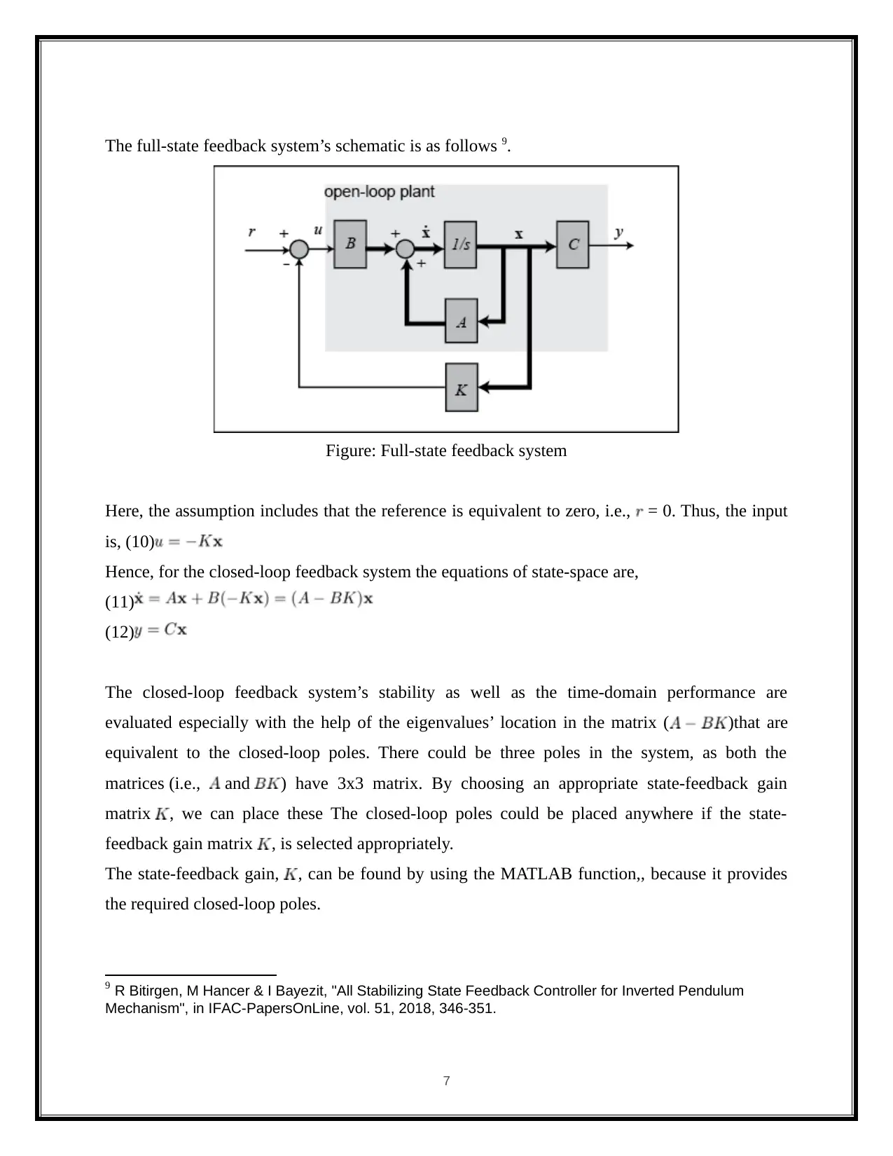
The full-state feedback system’s schematic is as follows 9.
Figure: Full-state feedback system
Here, the assumption includes that the reference is equivalent to zero, i.e., = 0. Thus, the input
is, (10)
Hence, for the closed-loop feedback system the equations of state-space are,
(11)
(12)
The closed-loop feedback system’s stability as well as the time-domain performance are
evaluated especially with the help of the eigenvalues’ location in the matrix ( )that are
equivalent to the closed-loop poles. There could be three poles in the system, as both the
matrices (i.e., and ) have 3x3 matrix. By choosing an appropriate state-feedback gain
matrix , we can place these The closed-loop poles could be placed anywhere if the state-
feedback gain matrix , is selected appropriately.
The state-feedback gain, , can be found by using the MATLAB function,, because it provides
the required closed-loop poles.
9 R Bitirgen, M Hancer & I Bayezit, "All Stabilizing State Feedback Controller for Inverted Pendulum
Mechanism", in IFAC-PapersOnLine, vol. 51, 2018, 346-351.
7
Paraphrase This Document
Need a fresh take? Get an instant paraphrase of this document with our AI Paraphraser
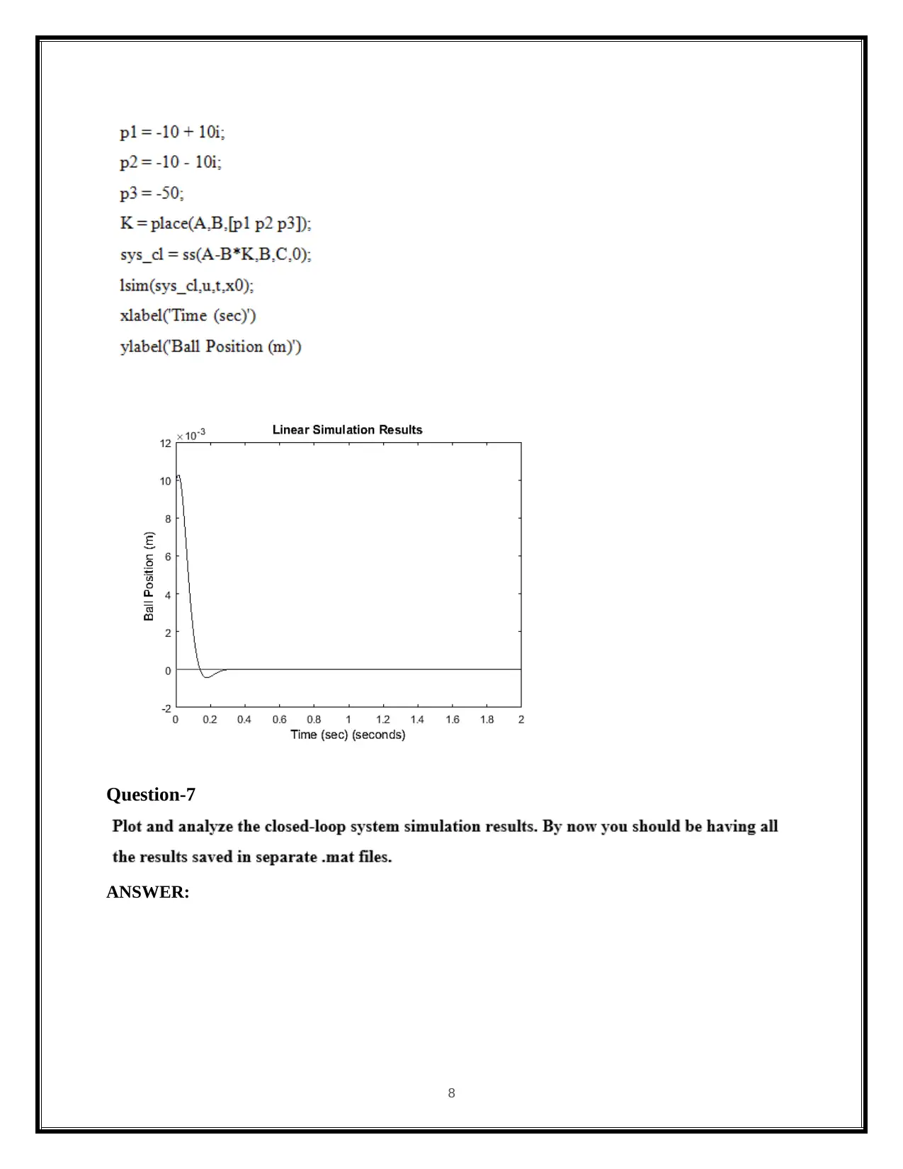
Question-7
ANSWER:
8
ANSWER:
8
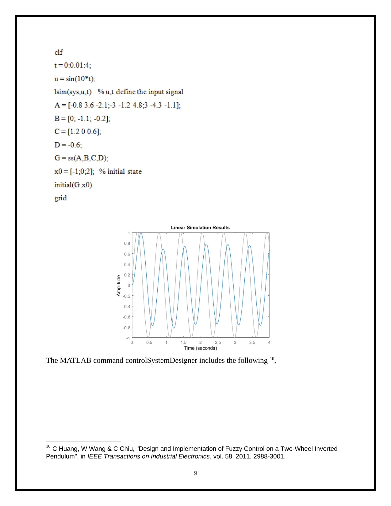
The MATLAB command controlSystemDesigner includes the following 10,
10 C Huang, W Wang & C Chiu, "Design and Implementation of Fuzzy Control on a Two-Wheel Inverted
Pendulum", in IEEE Transactions on Industrial Electronics, vol. 58, 2011, 2988-3001.
9
10 C Huang, W Wang & C Chiu, "Design and Implementation of Fuzzy Control on a Two-Wheel Inverted
Pendulum", in IEEE Transactions on Industrial Electronics, vol. 58, 2011, 2988-3001.
9
⊘ This is a preview!⊘
Do you want full access?
Subscribe today to unlock all pages.
Trusted by 1+ million students worldwide
1 out of 31
Related Documents


Your All-in-One AI-Powered Toolkit for Academic Success.
+13062052269
info@desklib.com
Available 24*7 on WhatsApp / Email
![[object Object]](/_next/static/media/star-bottom.7253800d.svg)
Unlock your academic potential
Copyright © 2020–2026 A2Z Services. All Rights Reserved. Developed and managed by ZUCOL.